
Abstract
This study tested the hypothesis that soil organic carbon (SOC) and total nitrogen (TN) spatial distributions show clear relationships with soil properties and vegetation composition as well as climatic conditions. Further, this study aimed to find the corresponding controlling parameters of SOC and TN storage in high-altitude ecosystems. The study was based on soil, vegetation and climate data from 42 soil pits taken from 14 plots. The plots were investigated during the summers of 2009 and 2010 at the northeastern margin of the Qinghai–Tibetan Plateau. Relationships of SOC density with soil moisture, soil texture, biomass and climatic variables were analyzed. Further, storage and vertical patterns of SOC and TN of seven representative vegetation types were estimated. The results show that significant relationships of SOC density with belowground biomass (BGB) and soil moisture (SM) can be observed. BGB and SM may be the dominant factors influencing SOC density in the topsoil of the study area. The average densities of SOC and TN at a depth of 1 m were about 7.72 kg C m−2 and 0.93 kg N m−2. Both SOC and TN densities were concentrated in the topsoil (0–20 cm) and fell exponentially as soil depth increased. Additionally, the four typical vegetation types located in the northwest of the study area were selected to examine the relationship between SOC and environmental factors (temperature and precipitation). The results indicate that SOC density has a negative relationship with temperature and a positive relationship with precipitation diminishing with soil depth. It was concluded that SOC was concentrated in the topsoil, and that SOC density correlates well with BGB. SOC was predominantly influenced by SM, and to a much lower extent by temperature and precipitation. This study provided a new insight in understanding the control of SOC and TN density in the northeastern margin of the Qinghai–Tibetan Plateau.
Export citation and abstract BibTeX RIS

Content from this work may be used under the terms of the Creative Commons Attribution-NonCommercial-ShareAlike 3.0 licence. Any further distribution of this work must maintain attribution to the author(s) and the title of the work, journal citation and DOI.
1. Introduction
Soils play an important role in the global carbon cycle. The soil organic carbon (SOC) pool has been estimated to be approximately three times the size of the atmospheric pool, and about four times the size of the biotic pool (Janzen 2004, Lal 2004). Minor changes in SOC storage could result in a significant alteration of atmospheric CO2 concentration (Davidson and Janssens 2006, Post et al 2009). Climate warming may have its largest positive feedback effects in high-latitude ecosystems that contain large pools of partially decomposed soil carbon accumulated under cold and moist conditions (Melillo et al 2002). A recent study (Tarnocai et al 2009) reported that the northern permafrost region contains approximately 1670 Pg of SOC, which accounts for approximately 50% of the estimated global belowground organic carbon pool. If these soils undergo both warming and drying, they have the potential to lose large amounts of carbon as CO2/CH4 to the atmosphere (Davidson et al 2000). Similarly, soils in high-altitude ecosystems have also been considered to play an important role in the global SOC cycle due to their high SOC density (Davidson and Janssens 2006). High-altitude soils play a critical role in the global terrestrial carbon cycle due to low temperature and potential sensitivity to climate warming (Davidson and Janssens 2006, Zimov et al 2006, Yang et al 2008, Post et al 2009, Schuur et al 2009).
A better understanding of the patterns and controls of SOC storage in high-altitude ecosystems is important to evaluate soil roles in the global terrestrial carbon cycle and potential feedbacks to global climatic change (Baumann et al 2009, Yang et al 2010). Many studies have addressed the characteristics of SOC pools and their control factors in high-altitude ecosystems. Studies include the soil C stock (Wang et al 2002, Tian et al 2007, Yang et al 2008) and its change trends (Piao et al 2006, Tan et al 2010), as well as CO2 flux (Xu et al 2005, Kato et al 2006). However, due to limited field observations and large spatial heterogeneity, the storage and distribution patterns of SOC in high-altitude ecosystems remain largely uncertain (Tao et al 2006, Yang et al 2008). The latter may be caused by a number of environmental factors showing high variations across a landscapes at large and small spatial scales. Variations include low temperature, permafrost, soil texture, and waterlogging (Hobbie et al 2000, Schuur et al 2008, Yang et al 2010). Therefore, extensive field soil surveys are expected to provide improved assessments of SOC storage, as well as vertical and spatial patterns of SOC.
The Qinghai–Tibetan Plateau (QTP), with its unique vegetation types and climate conditions, is the largest high-altitude ecosystem on earth. It represents an ideal region for the study of carbon cycles and the corresponding feedback interactions to global climatic change. Spatial distribution and temporal dynamics of SOC storage have been partly researched in this region (Wang et al 2002, Tao et al 2006, Yang et al 2010). However, few studies in the QTP ecosystem have addressed the vertical distribution of SOC (Tao et al 2006), total nitrogen (TN) and its stoichiometry (C:N ratio), and the environmental controls of the above-stated features (Tian et al 2007, Baumann et al 2009, Yang et al 2010). All of the above-described studies focused on the central QTP, while little work has been done on the northeastern margin of the QTP. The northeastern margin of the QTP is mainly influenced by the Asian monsoon system, the influence of which decreases westwards. The relatively moist and warm tropical Indian monsoon coming from the south is held back by big east–west stretching mountain ranges. Accordingly, there is a relatively high annual temperature (Xie et al 2010) and low precipitation in comparison to the characteristics of the southeastern QTP. Moreover, the geomorphological situation consists of complex mountain topography (Sheng et al 2010) compared to vast flat plateau-like areas interrupted by mountain ranges in the central QTP. The combined climate and topography conditions of the northeastern QTP give the region a large range of vegetation and soil types (Chen et al 2011).
Previous studies have reported significant climate warming in this area over the past 30 years (see e.g. Zhao et al 2004). Further, in the past 15 years, large areas of frozen soil have seriously degraded (Xie et al 2010). This has had a great impact on the soil environment and vegetation composition. Specifically, active layer thickness and soil temperature changes in permafrost altered the transfer processes of soil temperature and water conditions. Consequently, the stability of the vegetation and soil environment in the northeastern QTP was affected (Zhang et al 2003, Qin and Ding 2009, Yi et al 2011). The working hypothesis for this study was that SOC and TN distributions show clear relationships with selected soil parameters, vegetation composition, and climatic conditions. We then established SOC and TN density for each vegetation type and estimated SOC and TN storage. Overall, we examined how environmental factors affect the vertical distributions and spatial patterns of SOC and TN density.
2. Materials and methods
2.1. Study location and site description
The study area is located in the upstream regions of the Shule River Basin on the northeastern margin of the QTP. Altitudes range from 2100 to 5750 m, and the study region has an area of ∼ 1.25 × 10⁴ km2 (Xie et al 2010). This area belongs to the continental arid desert climate region. It has low average annual temperatures, little rainfall, and high evaporation (Sheng et al 2010). The mean annual temperature is approximately –5 °C the annual precipitation range is ∼100–300 mm (Chen et al 2011), and annual evaporation is about 1200 mm (Xie et al 2010). Due to the indirect influence of glaciers in the region, significant small scale temperature and precipitation gradients were observed, especially at the four plots in the northwestern part of study area (table 1). Our sampling campaign was conducted along a transect that traversed the typical vegetation and soil types within the study area. A total of 14 plots were selected among the gradients (figure 1). Plots SB1 and SB2 are located outside the boundary of the upstream regions of the Shule River Basin. We chose these plots because of their good accessibility and similarity in terms of vegetation characteristics and soil texture distributions to those throughout the boundary area.
Table 1. Dominant plants, soil type, mean annual temperature (MAT), mean annual precipitation (MAP) of different vegetation types. ASM: alpine swamp meadow; DG: desertified grassland; AM: alpine meadow; D: desert; DS: desert steppe; AS: alpine steppe; PV: periglacial vegetation.
| Vegetation types (area, km2) | Sampling plots | Dominant plants (Chen et al 2011) | Soil types | MAT (°C) | MAP (mm) |
|---|---|---|---|---|---|
| ASM (227) | SLP3 | Kobresia tibetica, Carex parva | Bog soils | −4.5 | 417 |
| DG (598) | SLP9 | Saussurea arenaria, Ajania pallasiana | Cold calcic soils | −4.8 | 422 |
| AM (803) | SLP1 | Kobresia capillifolia, Carex moorcroftii | Felty soils | −4.7 | 19 |
| SLP4 | Carex moorcroftii, Stipa purpurea | Frigid calcic soils | −4.8 | 417 | |
| SLP5 | Kobresia robusta, Artemisia nanschanica | Cold calcic soils | −5.2 | 400 | |
| SLP2 | Kobresia pygmaea, Carex moorcroftii | Cold calcic soils | −6.0 | 476 | |
| D (182) | SB1 | Salsola passerina, Allium spp. | Gray-brown desert soils | 6.3 | 67 |
| DS (3174) | SB2 | Stipa breviflora, Artemisia hedinii | Brown pedocals | 2.7 | 89 |
| AS (1794) | SLP6 | Stipa purpurea, Saussurea arenaria | Frigid calcic soils | −4.3 | 400 |
| SLP7 | Stipa purpurea, Leymus secalinus | Frigid calcic soils | −3.5 | 368 | |
| SLP8 | Stipa purpurea, Leontopodium leontopodioides | Cold calcic soils | −2.5 | 324 | |
| SB3 | Stipa purpurea, Leontopodium leontopodioides | Cold calcic soils | −0.3 | 168 | |
| PV (5674)a | SB4 | Rhodiola quadrifida, Poa annua | Frigid frozen soils | −5.0 | 205 |
| SB5 | Poa annua, Saussurea arenaria | Frigid frozen soils | −5.6 | 209 |
2.2. Soil samples collection and analysis, and biomass survey
To estimate SOC and TN storage and patterns in typical vegetation types within the altitude gradients, we sampled 42 soil pits from 14 plots (i.e., two or three soil pits at each plot). The plots were located at the northeastern margin of the QTP (figure 1), and sampling occurred during the summer months (July and August) of 2009 and 2010. At each sampling plot, three soil pits were excavated to collect samples for analyses of soil physical and chemical properties. Soil samples of each pit were collected schematically at depths of 0–10, 10–20, 20–30, 30–40, 40–60, 60–80 and 80–100 cm. Five subsamples for each depth layer were randomly collected and mixed into a composite sample, then packed in bags and brought to the laboratory. In the sample plot, three replicates of volumetric soil samples for each soil depth were collected using a cutting ring (volume of 100 g cm−3) to determine bulk density. Soil moisture (SM) was measured gravimetrically after 24 h drying at 105 °C. The volume of rock fragments (coarser than 2 mm) was determined by submerging moist rock fragments and recording the volume of displaced water. For larger rock fragments (>50 mm), volume was determined by visual estimation.
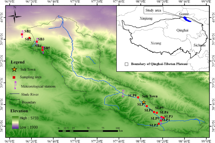
Figure 1. Spatial distribution of sampling sites of typical vegetation in the upper area of the Shule River Basin.
Download figure:
Standard imageSoil samples were air-dried and then hand-sieved through a 2 mm screen to remove roots, litter and stone. A subsample of the air-dried sample was ground to pass through a 0.25 mm sieve and was then analyzed for SOC and TN. SOC was determined by dichromate oxidation using the Walkley–Black procedure (Nelson and Sommers 1982). TN was measured using the micro-Kjeldhal procedure (ISSCAS 1978). Soil particle size distribution was determined by the wet sieve method (Chaudhari et al 2008).
All plants in five quadrats (0.5 m × 0.5 m) at each plot were harvested to measure aboveground biomass (AGB). Because recent studies have shown that 90% of roots in alpine grasslands are concentrated in the top 30 cm (Yang et al 2009, Chen et al 2011), we collected the belowground biomass (BGB) only to a depth of 0–40 cm. At each plot, BGB were drilled with an auger at depths of 0–10, 10–20, 20–30 and 30–40 cm. Each sample was repeated five times. Stones and other debris were removed, and the samples were packed in bags and brought to the laboratory. Each soil section was washed with a different pore-size sieve. Biomass samples were oven-dried at 80 °C to a constant weight. BGB was determined by the sum of biomass at depths of 0–10, 10–20, 20–30 and 30–40 cm.
We took photos of each plot using a multi-spectral camera before collecting biomass, to obtain NDVI values, using Tetracam Agricultural Digital Camera (ADC, Tetracam Inc., Chatsworth, CA, USA), with resolution of 2048 pixels × 1536 pixels. The ADC records three bands, i.e. near infrared, red and green, which are approximately equal to the fourth, third and second bands of the Landsat thematic mapper (TM). The pictures were then processed using a calibration file (the file was provided by ADC company according to measured reflectance values of green (G), red (R) and near infrared (NIR) for our multi-spectral pictures) in PixelWrench2 software. NDV I = (NIR − R)/(NIR + R) were further derived (Yi et al 2011).
2.3. Climate data, vegetation composition and soil types
Datasets of mean annual temperature (MAT) and mean annual precipitation (MAP) were derived from the climatic data of the northeastern margin of the QTP for the period of 2008–10. Data corresponding to the five plots were obtained and spatially interpolated from records of a nearby meteorological station (figure 1). Based on NDVI values for each vegetation type, vegetation types (figure 2) were grouped using a vegetation map interpreted by TM remote sensing data acquired on 16 July 2010. We selected seven typical vegetation types as being representative of the sampling sites to examine differences in vertical distributions of SOC, TN and C:N stoichiometry among the distinct vegetation types. Vegetation type and its size, dominant plants, soil type and climate are shown in table 1. The spatial distribution of vegetation types in the northeastern margin of the QTP is complex; however, it is related to corresponding precipitation and temperature conditions. More details of the representative plants have been described in Chen et al (2011). Generally, those soils may be described by their young development and strong degradation features, which are triggered by cryogenic processes or soil erosion. Consequently, a broad variety of soil formation factors is evident in the study area. According to the Chinese soil classification system, the main soil types in this area were (soil types according to WRB classification (IUSS Working Group WRB 2006) are given in parentheses): frigid calcic soils (Chernozems, Kastanozems); bog soils (gleysols, histosols, gelic gleysols, gelic histosols, umbric cambisols); brown pedocals (leptic to haplic cambisols); gray-brown desert soils (regosols (arenosols and leptosols)); frigid frozen soils (cryosols, gelic cambisols, gelic histosols); cold calcic soils (kastanozems); and felty soils (kastanozems or cambisols, frequently with felty turf-like topsoil). These felty turf-like topsoils contain large amounts of organic residuals and are widespread in cold alpine meadow areas (Kaiser 2004). The soil type data set (figure 2) was provided by Environmental and Ecological Science Data Center for West China, National Natural Science Foundation of China (http://westdc.westgis. ac.cn).
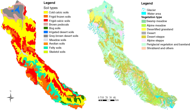
Figure 2. Distribution of vegetation and soil types in the research area of the northeastern QTP.
Download figure:
Standard image2.4. Vertical distribution of SOC and TN
The calculation of SOC density for each soil profile was obtained using equation (1).

where SOCD, hi, BDi, SOCi, and Ci are SOC density (kg m−2), soil thickness (cm), bulk density (g cm−3), SOC (g kg−1), and volume percentage of the soil particles fraction > 2 mm at layer i, respectively. Vertical distribution of TN was described analogously. The SOC density for each interval in the top 1 m were summed, and then to be multiplied by area of each vegetation type to obtain the storage of SOC and TN, and last the storage of SOC and TN for each vegetation type (seven typical vegetation types) to be summed to obtain the total study area SOC and TN storage. The C:N ratios were calculated using mass ratios.
Each dataset of topsoil (0–20 cm) was split into the two sampling depths (0–10, 10–20 cm), and statistical analysis was utilized with the 28 sample sizes. Linear regression and correlation analyses were conducted to evaluate the relationship between SOC content and soil acidity (pH), bulk density, SM, altitude, MAT, MAP, soil texture, AGB and BGB. A general linear mode (GLM) was used to describe the effects of the dependent parameters (vide supra) on the independent variables (SOC and TN density). These single condition models were used to investigate the impact of each dependent variable based on correlation analysis and multiple linear model explanation. The statistical analyses were conducted with SPSS software (version 11.5) and SAS software package (version 8.2). The P < 0.05 level was considered to be significant.
3. Results
3.1. Storage of SOC and TN
AGB, BGB and SOC density for all vegetation types are listed in table 2. As shown, AGB and BGB exhibited large differences among the vegetation types. Average SOC densities ranged from 4.39 to 19.84 kg m−2 for a thickness of 1 m in the different vegetation types. Within the study area, the total C and N storage in the top 1 m were about 96.08 Tg (1 Tg = 1012 g) and 11.61 Tg, respectively. According average densities were 7.72 kg C m−2 and 0.93 kg N m−2. In addition, average SOC densities were 8.11, 19.84, 7.09, 4.39, 9.24, 8.39 and 6.13 kg m−2 for a thickness of 1 m in frigid calcic soils, bog soils, brown pedocals, gray-brown desert soils, frigid frozen soils, cold calcic soils and felty soils, respectively (table 3).
Figure 3 illustrates the SOC and TN density in soil profiles for each vegetation type. The proportions of SOC below the 40 cm soil layer were 25%, 28% and 23% for alpine swamp meadow, desertified grassland and alpine meadow. Both SOC and TN density in different vegetation soils decreased as soil depth increased (figure 3). Similarly, a higher proportion of TN density in the upper layer was observed in all of the vegetation type soils. The average values for the seven different vegetation types were about 43% of total SOC and about 39% of total TN at 0–20 cm soil depth (figure 4). Soil C:N ratios ranged from 5 to 11 and exhibited a decreasing trend with soil depth in most vegetation types. However, the C:N ratios were relatively smooth in desertified grassland and desert (figure 5).
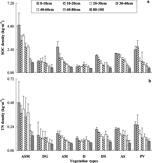
Figure 3. Soil organic carbon (SOC) density (a) and total N (TN) density (b) in soil profiles of different vegetation types. (ASM: alpine swamp meadow, DG: desertified grassland, AM: alpine meadow, D: desert, DS: desert steppe, AS: alpine steppe, PV: periglacial vegetation). Error bars express standard deviation from the mean.
Download figure:
Standard image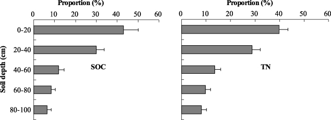
Figure 4. Averaged profiles (all vegetation types) for SOC and TN proportional distributions in the top 100 cm of soil in the northeastern margin of the QTP. Error bars express standard deviation from the mean.
Download figure:
Standard imageTable 2. SOC density (SOCD) and TN density (TND), aboveground biomass (AGB) and belowground biomass (BGB) in the top 1 m of different vegetation types.
| Vegetation types | SOCD (kg m−2) | TND (kg m−2) | AGB (g m −2) | BGB (0–10, 10–20 cm)a (g m −2) |
|---|---|---|---|---|
| Alpine swamp meadow (ASM) | 19.84 ± 1.81 | 2.34 ± 0.55 | 168.48 ± 0.94 | 12 261.09 ± 299.20 (66%, 19%) |
| Desertified grassland (DG) | 6.24 ± 1.73 | 0.75 ± 0.29 | 16.27 ± 5.95 | 472.78 ± 165.40 (47%, 52%) |
| Alpine meadow (AM) | 8.70 ± 1.19 | 0.81 ± 0.08 | 54.29 ± 9.21 | 1391.27 ± 599.17 (75%, 17%) |
| Desert (D) | 4.39 ± 0.71 | 0.68 ± 0.06 | 107.18 ± 26.71 | 1006.21 ± 506.61 (51%, 31%) |
| Desert steppe (DS) | 7.09 ± 0.65 | 0.99 ± 0.14 | 41.86 ± 3.06 | 1860.35 ± 171.43 (64%, 22%) |
| Alpine steppe (AS) | 9.24 ± 1.11 | 1.07 ± 0.21 | 56.42 ± 48.43 | 1505.79 ± 344.29 (65%, 21%) |
| Periglacial vegetation (PV) | 9.46 ± 1.77 | 1.15 ± 0.16 | 70.58 ± 26.27 | 819.97 ± 40.94 (62%, 26%) |
aThe values in brackets were the proportions of BGB in the 0–10 cm and 10–20 cm layer relative to the content of the entire 40 cm soil layer for each vegetation type, respectively.
Table 3. SOC density (SOCD) and TN density (TND) in the top 1 m of different soil types.
| Soil types (Chinese soil classification) | SOCD (kg m−2) | TND (kg m−2) |
|---|---|---|
| Frigid calcic soils | 8.11 ± 1.25 | 0.84 ± 0.16 |
| Bog soils | 19.84 ± 1.81 | 2.34 ± 0.55 |
| Brown pedocals | 7.09 ± 0.65 | 0.99 ± 0.14 |
| Gray-brown desert soils | 4.39 ± 0.71 | 0.68 ± 0.06 |
| Frigid frozen soils | 9.46 ± 1.77 | 1.15 ± 0.16 |
| Cold calcic soils | 8.39 ± 1.67 | 0.96 ± 0.14 |
| Felty soils | 6.13 ± 1.72 | 0.80 ± 0.01 |
3.2. Relationship of SOC with biomass, soil moisture, soil texture and climatic variables
A significant relationship between SOC density and SM (0–20 cm) was characterized by a linear function of SOC = 0.12 × moisture + 2.42 (R = 0.71, P < 0.01, n = 14). The correlation matrix for the 14 plots variables show significant correlations between SOC content in the topsoil (0–10 and 10–20 cm) and BGB (R = 0.73, P < 0.01). There was a significant relationship between SOC in the topsoil and AGB (R = 0.44, P = 0.02) (table 4). As an indicator for soil development processes, soil texture correlates with SOC and TN, showing a significant relationship between SOC content and soil clay fraction (R = 0.54, P < 0.01). There is a significant relationship between BGB and SM (R = 0.69, P < 0.01). The best-fit model of the GLM regression can be expressed as follows:


With the exception of SM, soil clay fraction and AGB, no other variables were included in the GLM. The SM (accounted for 54% of variation) was the most important parameter for SOC content, whereas the soil clay fraction (accounted for 43% of variation) was the most important parameter for TN content.
Table 4. Correlation matrix for the fourteen plots variables (soil parameter dataset was split into two sampling depths: 0–10 and 10–20 cm). (Note: SOC: soil organic carbon; TN: total nitrogen; BD: bulk density; SM: soil moisture; MAT: mean annual temperature; MAP: mean annual precipitation; AGB: aboveground biomass; BGB: belowground biomass; *, ** indicate significant effects at p < 0.05 and 0.01, respectively.)
| SOC (g kg −1) | TN (g kg −1) | pH value | BD (g cm −3) | SM (%) | Altitude (m) | MAT (°C) | MAP (mm) | Sand (%) | Silt (%) | Clay (%) | AGB (kg m−2) | BGB (kg m −2) | |
|---|---|---|---|---|---|---|---|---|---|---|---|---|---|
| SOC (g kg−1) | 1 | ||||||||||||
| TN (g kg−1) | 0.93** | 1 | |||||||||||
| pH value | −0.10 | −0.16 | 1 | ||||||||||
| BD (g cm−3) | −0.19 | −0.27 | 0.19 | 1 | |||||||||
| SM (%) | 0.71** | 0.69** | −0.06 | −0.12 | 1 | ||||||||
| Altitude (m) | 0.29 | 0.14 | 0.16 | 0.39* | 0.44* | 1 | |||||||
| MAT (°C) | −0.26 | −0.11 | −0.14 | −0.41* | −0.47* | −0.99** | 1 | ||||||
| MAP (mm) | 0.07 | −0.02 | 0.03 | 0.33 | 0.48** | 0.69** | −0.79** | 1 | |||||
| Sand (%) | −0.11 | −0.31 | 0.17 | 0.46* | −0.10 | 0.66** | −0.65** | 0.40* | 1 | ||||
| Silt (%) | −0.08 | 0.11 | −0.12 | −0.46* | −0.09 | −0.72** | 0.72** | −0.49** | −0.96** | 1 | |||
| Clay (%) | 0.54** | 0.69** | −0.23 | −0.31 | 0.52** | −0.27 | 0.25 | −0.05 | −0.75** | 0.54** | 1 | ||
| AGB (kg m−2) | 0.44* | 0.46* | −0.01 | 0.02 | 0.33 | −0.05 | 0.06 | −0.20 | 0.30 | −0.13 | 0.12 | 1 | |
| BGB (kg m−2) | 0.73** | 0.72** | −0.01 | −0.15 | 0.69** | 0.18 | −0.20 | 0.05 | 0.51** | 0.05 | −0.08 | 0.58** | 1 |
3.3. Relationship of SOC and climate variables in the four vegetation types of the northwestern region of the study area
For the following vegetation types in the northwestern part of the study area: desert (SB1), desert steppe (SB2), alpine steppe (SB3) and periglacial vegetation (SB4) (figure 1), the proportion of SOC below the 40 cm soil layer decreased as temperature decreased and precipitation increased (desert > desert steppe > alpine steppe > periglacial vegetation). SOC density in the topsoil decreased as temperature increased, but increased as precipitation increased. Correlations of SOC with climate parameters diminished as soil depth increased (table 5).
Table 5. Correlations between the vertical distribution of SOC density and climatic variables of four vegetation types (D, DS, AS and PV) with significant climatic gradients. (Note: MAT: mean annual temperature; MAP: mean annual precipitation; Y: total SOC density for given soil depth; X1: temperature; X2: precipitation; R is correlation coefficient; * indicates significant effects at p < 0.05.)
| Depth (cm) | MAT | MAP | ||
|---|---|---|---|---|
| Linear equation (Y) | Correlation coefficient (R) | Linear equation (Y) | Correlation coefficient (R) | |
| 0–20 | − 0.32X1 + 3.65 | 0.97* | 0.02X2 + 0.35 | 0.93* |
| 0–60 | − 0.44X1 + 6.99 | 0.86 | 0.03X2 + 2.03 | 0.90 |
| 0–100 | − 0.46X1 + 8.19 | 0.85 | 0.04X2 + 2.99 | 0.89 |
4. Discussion
4.1. SOC and TN storage estimation and their significance
The total of C and N storage for the top 1 m were approximately 96.08 and 11.61 Tg in the upstream regions of the Shule River Basin in the northeastern margin of the QTP. Further, the average density of SOC was 7.72 kg m−2, which was higher than the average density of 6.52 kg m−2 for the whole QTP (Yang et al 2008). We found the lowest SOC density of 4.39 kg m−2 in areas with desert (D) vegetation type (gray-brown desert soils) (table 2). This was lower than the average value for desert globally (6.20 kg m−2) (Jobbágy and Jackson 2000), while both densities were higher than the average SOC density of gray-brown desert soils (1.24 kg m−2) in Qinghai Province (Wang et al 2002). The highest SOC density was found in alpine swamp meadow (19.84 kg m−2). This value was lower than that in the central QTP (49.88 kg m−2) (Wang et al 2002) with the same soil type of bog soil. Wu et al (2003) have reported an average SOC density of 9.47 kg m−2 in China's alpine meadow vegetation, whereas Yang et al (2008) published an average SOC density of 9.05 kg m−2 for the alpine meadows in the whole QTP. Both of the above recorded density values for alpine meadows were higher than those found in our study (8.70 kg m−2). However, for alpine steppe, Wu and Yang reported lower SOC densities (7.48 and 4.38 kg m−2) than the densities we found (9.24 kg m−2). These differences could be an effect of the significant spatial heterogeneity across the QTP (Baumann et al 2009). Although the vegetation type was uniform, soil types and climate conditions were very different, thus playing a critical role in determining the SOC density distributions (Ravindranath and Ostwald 2008). Further, our study concentrates on the northeastern margin of the QTP. Previous studies involve several uncertainties for average C density estimation of different vegetation types of the QTP, such as limited data to extrapolate over large areas and use different geostatistical algorithms (Wang et al 2002, Yang et al 2008). This indicates that an estimation of SOC storage for the entire QTP requires more field data and a finer sampling raster.
4.2. Vertical distributions of SOC, TN
The proportions of the first 0–20 cm interval related to the total content of the 1 m profile (43% of total SOC and 39% of total TN) are lower than the comparable proportions that Yang et al (2010) found in alpine grasslands on the central QTP (49% of total SOC and 43% of TN) (figure 4). The results of our study are consistent with those published by Jobbágy and Jackson (2000) (42% and 38% for SOC and TN at global ecosystems, respectively). The distribution of SOC and TN concentrated in the surface soil layer could be caused by their shallower root distribution (Jobbágy and Jackson 2000, Yang et al 2010). The distribution of relative BGB in 0–10 cm and 10–20 cm in this study (table 2) also supports this hypothesis. Due to this shallow root allocation in alpine ecosystems (see e.g. Yang et al 2009), comparably little SOC can be sequestered in deeper soil layers. Consequently, SOC storage in deep layers can be not as high as in woodland ecosystems (see e.g. Sommer et al 2000). In other words, because of even higher inputs of organic material, SOC and TN levels are generally concentrated in topsoil (Li and Zhao 2001).
The vertical distribution of SOC for the seven vegetation types generally showed that SOC density in 20 cm interval decreased as soil depth increased (figure 3). This agrees with observations on the entire QTP (Yang et al 2010), and with those of other ecosystems (Jobbágy and Jackson 2000). However, the soil depth of 20–40 cm revealed the highest SOC density (the sum of SOC density in 20–30 and 30–40 cm soil layer) in desert-type vegetation (figure 3). Litter fallen on the soil surface and turnover of fine roots are regarded as the main pathways of SOC input in natural ecosystems (Li and Zhao 2001). Thus potential explanations for this high SOC content include: (1) a small amount of AGB input; and the BGB inputs in the 20–40 cm soil layer were similar to those of the 0–20 cm layer in desert-type vegetation (data not shown); and (2) more organic matter was decomposed in the topsoil with relatively higher temperature and lower precipitation in desert-type vegetation soils (table 1). Another possible reason is the frequently observed high sediment input (e.g. aeolian sedimentation), where fine sand and silts are deposited on top, frequently burying the humic horizons of former soil formation underneath the fresh sediment.
Importantly, the above-described process of active aeolian sedimentation is closely linked to permafrost degradation. Such degradation is often triggered by direct (e.g. overgrazing, construction) (Zhang et al 2006, Dai et al 2011) and indirect (climate change) human impact. It hence not only helps to explain the occurrence of SOC in deeper soil layers at desert vegetation plots, but also provides evidence for the vertical distribution of plant available nutrients. The main parameters that have to be considered are dilution caused by the ongoing sediment input, and the changes in soil temperature and moisture regimes linked to decomposition of organic material (Baumann et al 2009). The latter are particularly important if permafrost is degraded, leading to a thicker active layer and consequently to lower SM contents in accordant relief positions.
4.3. C:N ratio and its vertical distributions
C:N ratios of most vegetation types (except desertified grassland and desert) displayed decreasing trends with increasing soil depth (figure 5), which was consistent with previous study results (Callesen et al 2007). This is because there is more recalcitrant material with slower decomposition rates and lower C:N ratios in deep soil than in topsoil (Post et al 1985, Trumbore 2000). The C:N ratios (mass ratio) in this study ranged from 5 to 11. This result was consistent with previous results for similar regional conditions in the eastern QTP in which C:N ratio ranged from 6 to 14 (Xue et al 2009). The overall C:N ratios for our study area (especially at 0–20 cm depth) were low, and were thus similar to results in the central QTP (Yang et al 2010), and slightly lower than results in the frigid highland climate zone of China (11.66 ± 0.94) (Tian et al 2008). However, C:N ratios in this study were far lower than C:N ratios (17.40) in frigid highland climate zones outside China, summarized from Post et al (1985). Post et al's high values may have resulted from some of the soil samples containing a humified litter layer that had a higher C:N ratio than soil (Tian et al 2008). Compared to the overall C:N ratios in frigid highland climate zones of China, our study area has relatively cold winters (freeze-thaw cycle) and warm summers (high temperature). This favors organic matter decomposition and nutrient release. Nevertheless, the low vegetation coverage in the northeast margin of the QTP (Xie et al 2010) implied the relatively low organic matter input. Therefore, we conclude that high mineralization ability and low amounts of litter returning in soil may be the cause of lower C:N ratios.
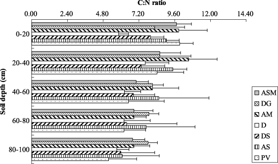
Figure 5. Variations of C:N ratios among the soil profiles of different vegetation types in the northeastern margin of the QTP (ASM: alpine swamp meadow, DG: desertified grassland, AM: alpine meadow, D: desert, DS: desert steppe, AS: alpine steppe, PV: periglacial vegetation). Error bars express standard deviation from the mean.
Download figure:
Standard image4.4. SOC density and its main influencing factors
SOC concentration depends on the balance between organic matter input and organic matter loss from soil (Zhuang et al 2007). Our results showed a higher correlation coefficient between SOC in the topsoil and BGB than between SOC and AGB, and a significant correlation between AGB and BGB (table 4). Although equation (2) indicated that AGB was a stable predictor for SOC content, BGB is most likely the main resource and dominant factor for SOC density in the topsoil in our study area. A study by Hui and Jackson (2006) reported that about 70% of net primary production of vegetation in alpine ecosystems is distributed in the belowground parts of plants. Consequently, these parts are an important source of SOC. In addition, our results showed that ratios of BGB:AGB were very high (with an average of 32). The high BGB:AGB ratio is an effect of long-term adaptation of alpine grasslands to extreme environments, a common feature of alpine grasslands all over the world (Mokany et al 2006). Therefore, when estimating SOC storage and its temporal dynamics in high-altitude grassland ecosystems, the influence of BGB on SOC is an important factor to examine.
Although more than 90% of BGB in alpine grasslands has been shown to be concentrated in the top 30 cm of soil (Yang et al 2009), about 27% of SOC was distributed lower than 40 cm in our investigation area (figure 4). Accordingly, the main part of BGB was distributed much closer to the surface than was SOC. This pattern was originally observed in humid grasslands (Weaver et al 1935) and has been confirmed in other grasslands (Jobbágy and Jackson 2000). Decreasing SOC turnover with depth (Trumbore 2000) implies higher SOC accumulation rates in deeper soil layers. Another important reason for these observations is the migration of SOC as a result of leaching, which can lead to C enrichment often consisting of a more persistent and stable soil C pool rather than close to the surface (Guggenberger and Kaiser 2003, Strahm et al 2009, Rumpel and Kögel-Knabner 2011).
Equation (2) indicated that SM was a stable predictor for SOC. Importantly, significant relationships between SOC density and SM (R = 0.71, P < 0.01) were evident on a landscape scale in our study. Other studies have also reported similar patterns of SOC interrelationships in high-altitude ecosystems (Hobbie et al 2000, Baumann et al 2009, Yang et al 2010). It is likely that higher SM, together with improved SOC quality, leads to higher plant productivity and substrate availability in ecosystems. Thus, this leads to higher SOC and TN contents in related soils (Schimel et al 1990, Reichstein et al 2003, Reichstein and Beer 2008). This is particularly so in potentially dry regions (Giardina and Ryan 2000).
Frozen soils and their degradation patterns have direct and indirect impacts on SM conditions, and consequently these patterns affect vegetation and carbon sequestration in periglacial environments. Permafrost degradation is directly associated with soil hydrology, leading to severe changes in soil moisture–temperature regimes, and hence affecting the nutrient supply of plants (Zhang et al 2003). Plant biomass productivity and community coverage (Jorgenson et al 2001, Wang et al 2007), and structure and function of vegetation (Cheng and Wang 1998) are all directly interrelated. There was no direct correlation between MAT and SOC (table 4), but there is a significant negative correlation between MAT and soil moisture. It implied that permafrost was a crucial factor to influence SM and SOC in study area. An increase in air temperature would cause the surface soil to be desiccated (as the permafrost degradation), which may result in a decrease of SOC in this region. In addition, vegetation would evolve to other species' composition, altering SOC storage and patterns. Consequently, differences in vertical distribution of SOC and TN as presented in our study help to better understand response and feedback mechanisms of SOC and TN in high-altitude ecosystems related to potential vegetation changes under the scope of global warming.
4.5. Decreasing influence of MAT and MAP on SOC with soil depth
In order to examine the relationship between SOC and climate variables, a subgroup of four vegetation types located in the northwestern part of our study area was selected (figure 1). Our results agree well with those published by Jobbágy and Jackson (2000) and Post et al (1982), showing that SOC density generally increases with increasing precipitation and decreasing temperature. Interestingly, we found high correlations of SOC with climatic factors in the top 0–20 cm, diminishing with the increase of soil depth (table 5). These findings are consistent with data from alpine ecosystems located in the central QTP (Tian et al 2007, Yang et al 2010). Other studies (Jobbágy and Jackson 2001, Tian et al 2007) have indicated that the importance of these controlling mechanisms changes with depth, thus climate effects are predominantly seen in layers close to the surface. This may be due to increasing proportions of slow-cycling SOC fractions in deep soil (Jobbágy and Jackson 2000, Rumpel and Kögel-Knabner 2011). Yang et al (2010) reported three reasons for this diminishing relationship: (1) slower-cycling SOC in deep soil layers; (2) soil buffering capacity reducing the effects of environmental influences in deep soil layers; and (3) a narrower range of SOC content in deep soil layers.
5. Conclusions
The SOC is concentrated in the topsoil and correlates well with BGB, which is the main resource and dominant parameter affecting SOC density in the topsoil. Moreover, SM retention is important for plant growth and ultimately for SOC formation in the study area. Soil texture is a critical factor for water retention in soil; e.g. sandy soils have low available water capacity and silty clay substrates have a high potential to hold water. According to our results, it can be assumed that SM is influenced even more by varying soil texture or the evidence of permafrost than by changing amounts of precipitation between years or over the main vegetation period. Degradation of permafrost under the scope of global warming leads to severe changes of SM conditions, and has a great influence on SOC storage patterns.
SOC in the upper parts of the topsoil is closely related to climatic factors (temperature and precipitation), and shows a diminishing relationship with soil depth in the four vegetation types of the northwestern study area. This indicates that SOC in the surface layer is vulnerable and should be strictly protected to minimize the risk of a potentially large carbon release. It is also important to mention that the dependent variables are interrelated, particularly SM and BGB.
Since decomposition of SOC is associated with permafrost degradation, feedback mechanisms between permafrost and soil water dynamics are key aspects of future development of the QTP ecosystem under climate change conditions. These feedback mechanisms are not yet sufficiently understood. Planned future work characterizing permafrost type and SOC pools at these plots (e.g. at 10 year intervals) will provide an opportunity to further assess vegetation and soil C dynamics.
Acknowledgments
This work was supported by the Global Change Research Program of China (2010CB951404), the National Natural Science Foundation of China (No. 41171054, 40901040), the Foundation for Excellent Youth Scholars, the Freedom Project (No. SKLCS-ZZ-2012-02-02) and the Open-Ended Fund (No. SKLCS 10-08) of the State Key Laboratory of Cryospheric Sciences, Cold and Arid Regions Environmental and Engineering Research Institute, Chinese Academy of Sciences, the China Postdoctoral Science Foundation (201104347). We are grateful to Professor Baisheng Ye for providing meteorological data. We thank the two anonymous reviewers for valuable suggestions and comments on the manuscript.