

Abstract
Global climate change (GCC) is projected to bring higher-intensity precipitation and higher-variability temperature regimes to the Northeastern United States. The interactive effects of GCC with anthropogenic land use and land cover changes (LULCCs) are unknown for watershed level hydrological dynamics and nutrient fluxes to freshwater lakes. Increased nutrient fluxes can promote harmful algal blooms, also exacerbated by warmer water temperatures due to GCC. To address the complex interactions of climate, land and humans, we developed a cascading integrated assessment model to test the impacts of GCC and LULCC on the hydrological regime, water temperature, water quality, bloom duration and severity through 2040 in transnational Lake Champlain's Missisquoi Bay. Temperature and precipitation inputs were statistically downscaled from four global circulation models (GCMs) for three Representative Concentration Pathways. An agent-based model was used to generate four LULCC scenarios. Combined climate and LULCC scenarios drove a distributed hydrological model to estimate river discharge and nutrient input to the lake. Lake nutrient dynamics were simulated with a 3D hydrodynamic-biogeochemical model. We find accelerated GCC could drastically limit land management options to maintain water quality, but the nature and severity of this impact varies dramatically by GCM and GCC scenario.
Export citation and abstract BibTeX RIS
1. Introduction
In the 'Age of the Anthropocene', changes in ecological systems are increasingly coupled with changes in social, economic and political systems [1, 2]. These coupled complex adaptive systems are broadly defined as 'Social Ecological Systems' (SESs) [3–7]. Social-ecological systems are complex adaptive systems characterized by threshold effects, path dependencies, nonlinear dynamics, multiple basins of attraction, and limited predictability [8]. Natural ecosystems often do not respond smoothly to gradual change [4], and may undergo sudden, threshold-based, nonlinear, long-lasting changes in structure and function [9, 10]. These nonlinear state transitions are amplified in SESs, where regime shifts in social-economic networks may result in rapid changes to resource utilization, resulting in dramatic variation in the stresses placed on ecological communities [4, 9]. Regime shifts in SESs can result in rapid state transitions in a variety of natural ecosystems, including coral reefs and fisheries [10–12], tropical forests and rangelands [13–17] among others. Of particular interest to the current study are well-documented state changes in freshwater lakes resulting from shifting land-use practices in lake catchments [18–28]. In the Lake Champlain Basin of Vermont, New York and Quebec, changes in agricultural activity resulting from evolving socio-economic pressures have resulted in increased nutrient loads to the lake, promoting a rapid shift to eutrophic conditions within significant portions of the lake [29]. The consequences of climate change contributing to the development of intractable eutrophic conditions may suggest that climate change impacts will outpace the land use management type of policy responses now in place in this region being enacted by EPA under the federal water quality act [53]. To understand this, a social-ecological systems approach to modeling these dynamics is needed.
To detect regime shifts in water systems, SES models have been developed using statistical approaches [10], system dynamic models [19, 30], equilibrium models [21] and to some extent process-based approaches; however, implementation of process-based SES models is frequently complicated by cross-scale incompatibilities in domain-specific models [4, 31]. This study aims to develop a computational SES modeling approach to simulate how the cross-scale dynamics of global climate change (GCC) (relatively slow) and regional land-use land cover change (LULCCs) (relatively fast) impact watershed scale hydrological systems (e.g. runoff) and downstream freshwater lakes and their bays (e.g. water quality indicators). Anthropogenic GCC will likely continue to induce higher intensity precipitation, and increase variability in both the precipitation and temperature of the North-Eastern United States [32, 33]. However, there is considerable variability in predictions from different global climate models (GCMs) under different greenhouse gas emission scenarios. It is therefore not clear how these climatic changes at global scales will couple with human induced LULCCs at regional scales to affect the dynamics of the hydrological system at watershed scales. Uncertainty in global scale GCMs, coupled with global green house gas mitigation scenario variability shown through differential representative concentration pathway (RCP) scenarios of IPCC [54], alters boundary conditions for regional scale watersheds and lakes. Usage of a single GCM or a single RCP in setting up policy and management goals at regional scales in the face of uncertainty at global scale dynamics poses fundamental challenges that require development of spatially sensitive and temporally nested computational SES models. This paper presents a proto-type for one of these cross-scale computational SES models, which we call a cascading integrated assessment model (IAM). This IAM is used to quantify the impact of the interaction of GCC induced temperature and precipitation variability with human-system induced LULCC on watershed nutrient loading and the frequency and severity of harmful algal blooms (HABs) in Missiquoi Bay of Lake Champlain for 2000–2040 timeframe under different GCM and RCP scenarios. The paper addresses the following overarching questions: What will be the coupled impacts of climate change and land use change on riverine nutrient loading to the lake and, when combined with direct climate driven changes to lake water temperature, how will water quality evolve under different RCP and GCM scenarios?
2. Methods
The cascading IAM (figure 1) is a spatio-temporal model that uses a complex adaptive systems computational approach to study the interactions of climate and LULCC in the Lake Champlain Basin. Statistical downscaling of four GCMs for three RCP scenarios was performed to generate a spatial grid of future temperature and precipitation (section 2.1). In parallel, an agent based model (ABM) simulated four extreme LULCC scenarios (section 2.2). Combinations of climate as well as four LULCC scenarios were used in a distributed hydrological model (RHESSys) to estimate river discharge and nutrient loading from the Missisquoi watershed into Lake Champlain (section 2.3). The nutrient dynamics in Lake Champlain is, in turn, simulated by high resolution hydrodynamic and biogeochemical lake models (A2EM) (section 2.4). The IAM output was calibrated with the USGS stream-flow gage data and water quality sensor data for a baseline scenario. We used the 'extreme world method' for alternate scenario generation to compare with the baseline scenario in the Missisquoi SES. The extreme world method captures the broadest possible range of relationships between critical uncertainties, predetermined trends and behaviors of individual and policy level actors in the system under study [59, 60]. The computational integration across models was undertaken in Pegasus (section 2.5).
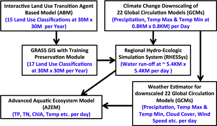
Figure 1. Schematic of the Missisquoi Basin IAM components (black boxes and text) illustrating example input variables and/or impact metric parameters (blue text) for each component, computationally connected (arrows) in a directed acyclic graph environment (Pegasus).
Download figure:
Standard image High-resolution image2.1. Climate change downscaling
We developed an ensemble of topographically downscaled, high-resolution (30'', ~1 km), daily maximum and minimum temperature (at 2 m above the surface) and precipitation simulations by applying an additional level of downscaling to the 1/8° (~12 km) bias correction with constructed analogs dataset (BCCA) [34], hereafter referred to as intermediately downscaled data. The process used high-resolution elevation and station observations, and consisted of four basic steps [35]: first, empirical relationships between surface temperature and elevation, and precipitation and elevation were derived. Second, the 1/8° intermediately downscaled GCM simulations were adjusted to a reference elevation (200 masl) using the derived relationships and a 1/8° digital elevation model (DEM). Third, the adjusted grids were interpolated to a grid with the resolution of 30''. Fourth, the 30'' interpolated data were topographically adjusted using the derived relationships and a 30'' DEM. The downscaled temperature and precipitation had a lower bias than the initial BCCA data when compared to station observations, especially for the higher elevation areas. The downscaling was particularly successful at decreasing the root mean standard deviation of temperature [35]. Additional methods details can be found in the supplementary materials [S1] and Winter et al [35]. The process was run for 63 climate ensemble members, comprising 21 intermediately downscaled GCMs and RCPs 4.5, 6.0 and 8.5. For the purposes of this paper, we chose four GCMs that bracket the range of expected changes in temperature and precipitation. To determine these four GCMs, we compared future trends among the available GCMs for RCP 8.5 and selected the GCMs with the highest and lowest changes in precipitation and average temperature. If one GCM ranked first in two categories, it was kept for one category and the next one ranked was chosen for the other category. We use bias-corrected GCM data, so temperature and precipitation across GCMs are approximately the same for the baseline period (1970–1999). The four GCMs therefore represent the greatest and least warming and largest increase and decrease in precipitation. The aim of this step was to select a subset of GCMs to maintain a manageable number of scenarios while creating a comprehensive set of potential extreme outcomes. We refer to these GCMs as: warm (MIROC-ESM-CHEM), cool (MRI-CGCM3), wet (NorESM1-M), and dry (IPSL-CM5A-MR) GCMs.
Relatively large uncertainty for projected changes in the temperature (figure 2(a)) and precipitation (figure 2(b)) for Missisquoi watershed exist. Using a 5 year average scale, the warm GCM predicted an average temperature increase of 3.6 ± 1 C by 2040 for RCP8.5, relative to the 1970–1999 baseline period. In contrast, the cold GCM only predicted a temperature increase of 1.2 ± 0.7 C. Similarly, the wet GCM predicted 0.35 ± 0.1 mm d−1 increase in precipitation for RCP8.5, while the dry GCM predicted 0.08 ± 0.31 mm d−1 increase in precipitation for RCP8.5. We note that changes in land use within the IAM do not impact the land use of climate projections. The land use for each individual climate projection is defined by the GCM itself.

Figure 2. (a) Four GCM projections for three RCP scenarios of temperature change in the Misssisquoi watershed (baseline = 1970–1999). (b) Four GCM projections for three RCP scenarios of precipitation change in the Missisquoi watershed (baseline = 1970–1999).
Download figure:
Standard image High-resolution image2.2. LULCC ABM
The framework of the LULCC ABM, shown in figure S1 of supplementary materials and explained in detail by Tsai et al [36] and Zia et al [37, 38] consisted of four procedures. First, the ABM initialized agents and parameters based on 2001 National Land Cover Database, zoning and economic development data. Agents were categorized into two major types: human agents, who made land use decisions in each time period given their perceived expected utilities; and land grid cell agents, which produced ecosystem services (ESs) that affected the human agents' expected utilities. Three types of human agents were modeled: agricultural, urban residence and business landowners. Second, the ABM evaluated the landowners' expected utilities for the current year based on ESs produced from agricultural landholding. The agricultural landowners' expected utilities positively correlated with ESs gained from managing their lands. The ESs provided by farmers' landholdings were expected to change corresponding to a land use transition. Given the level of the agricultural landowners' expected utilities, different land use decisions were made. When expected utility was small and landholdings were close to urban centers, farm lands were likely to be bought by developers and subsequently turned into urban lands, given that there was a demand for urban residences. Third, the ABM updated both the human and the land cell agents' properties and then re-categorized these agents based on their current properties. Last, the ABM generated simulated land use patterns for every year from 2001 to 2041.
Figure 3 shows four alternate LULCC scenarios derived for the focus watershed that might emerge in response to differential policy and human behaviors during the study period (see supplementary materials S2 for more information on calibration and validation procedures). The calibrated scenario for LULCC projects forward to 2041 allowing the evolution of land use without any major significant policy, economic or governance changes. Henceforth, we call the calibrated scenario increased economic disparity scenario. In contrast, the agriculture expansion scenario assumes significant investments in agriculture (both dairy and crop production), relaxation of current land-use conservation laws/policies, and increases in the main dairy and crop market prices, which lead to farmers' financial gains and, in turn, increase the fraction of farm land in the watershed. This is defined as large wealthy farmers' population (LWFP) scenario. On the other extreme, a forest conservation scenario, 2041 end-state shown in figure 3, assumes the opposite of agricultural expansion scenario: current land-use conservation laws/policies remain intact, main dairy and crop prices remain stagnant, and a sizeable fraction of farmers continue to suffer losses over time, which reduces farm land in the watershed over time compared with the calibrated scenario. The forest conservation scenario is characterized as large poor farmers' population (LPFP) scenario. Finally, the urbanization scenario assumes moderate expansion of urban areas with higher (than calibrated scenario) influx of population and an increase in the size of existing firms and addition of new firms operating in the urban regions that generate new jobs for urban residents (figure 3). The urbanization scenario is called increased development scenario. Given large path dependencies in LULCC, as well as shorter (40 years) simulation horizon, the net changes between agriculture, forest and urban cells within the watershed were relatively small (see table S1). Direct effects of climate change on LULCC are not modeled in this ABM.

Figure 3. Land-use classifications produced by the LULCC model for four economic and policy scenarios for the final simulation year (2041), also showing initial land-cover at start of simulation.
Download figure:
Standard image High-resolution image2.3. Physically based hydrological model (RHESSys)
The regional hydro-ecologic simulation system (RHESSys) model is a distributed hydrology model designed to simulate interactions between carbon and water fluxes, and climate patterns within a mountainous environment [39, 40]. We employed the RHESSys model here to examine the impacts of climate and LULCC on nutrient loadings within the Missisquoi River watershed. RHESSys combines both a set of physically based process models and a methodology for partitioning and parameterizing the landscape over spatially variable terrain (~10 m to hundreds of kilometers). The RHESSys hydrologic process models have been adapted from several pre-existing models and include snow accumulation and melt, interception, infiltration, transpiration, soil and litter interception, evaporation and shallow and deep groundwater subsurface lateral flow. For example, RHESSys uses the Penman Monteith method for evaporation and sublimation of intercepted water, transpiration and soil and litter evaporation processes [41]. RHESSys also uses the Jarvis model for stomatal conductance calculations based on air temperature, vapor pressure deficit, wind speed and other environmental factors such as light and CO2 [42]. The version of RHESSys used for this work includes both surface and subsurface storage routing and a deep groundwater store. Water is explicitly routed between spatial patches, representing spatial heterogeneity in soil moisture and lateral water flux to the stream (see supplementary materials S3 for calibration details). Figure 4 depicts the RHESSys performance during the calibration year. Simulated runoff results were able to explain about 62% of the variance observed in daily runoff during the calibration year (i.e. Nash Sutcliffe Efficiency = 0.62). The model overestimates the daily runoff by about 6% during the calibration years (i.e. 1998 water year). The annual precipitation amount over the study watershed during the calibrated water year is 1270 mm, and the total observed runoff at the watershed outlet is 755 mm.
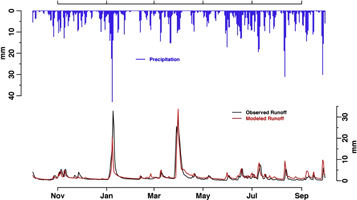
Figure 4. Daily simulated (red line) and observed (black line) runoff during the 1998 water year (October–September) for the Missisquoi River watershed at the USGS streamflow gauge # 04294000. Blue lines on the top give daily precipitation values aggregated over the Missisquoi watershed during the 1998 water year.
Download figure:
Standard image High-resolution image2.4. Advanced aquatic ecosystem model
The modeling framework chosen for Missisquoi Bay consisted of a 3D hydrodynamic model known as environmental fluid dynamics code (EFDC) [43, 44]; and a water quality model, row column AESOP (RCA) [55], containing an integrated sediment diagenesis submodel capable of tracking changes in sediment nutrient stores over time [56]. EFDC [43] is widely used and maintained by the US Environmental Protection Agency. EFDC uses a finite volume solution scheme for hydrostatic primitive equations on a staggered grid, and predicts water temperature, flow, and salinity based on meteorological forcing variables and hydrologic inputs. RCA is a water quality model that has been applied in a number of lake, river, and estuary studies to support management decision making [44–49]. This version of RCA has been modified to simulate up to 5 phytoplankton groups, in addition to carbon, oxygen, nitrogen, phosphorus, and silica dynamics, and other ecological processes that are not utilized here. Four phytoplankton groups were represented, approximating spring diatoms, summer eukayotes, non-N-fixing cyanobacteria, and N-fixing cyanobacteria. RCA also has an integrated sediment diagenesis subroutine based on the three G-class model [56], and has the ability to track sediment nutrient deposition, transformation, release, and burial over time. The sediment model consists of a 2-layer representation of the sediment, with a variable-depth oxygenated surface layer, the depth of which is driven by modeled sediment oxygen demand. The sediment model simulates partitioning of  between dissolved and particulate fractions as a function of sediment oxygen concentrations. Both EFDC and RCA have been modified by LimnoTech (Ann Arbor, MI) to allow cross-model compatibility and simulation of additional processes. The coupled EFDC-RCA model components are collectively referred to as the advanced aquatic ecosystem model (A2EM). A2EM was calibrated using 23 years of long-term monitoring data for temperature, total nitrogen, total phosphorus (TP), and chlorophyll-a (ChlA) at two sites within the bay, in addition to two years of comprehensive high-frequency biological, chemical, and hydrodynamic data collected as part of this study. Detailed description of model calibration is found in the supplemental material (S4.2 and figures S9–S15).
2.5. Model integration
The model interactions in figure 1 are transformed into an abstract computational workflow using the Pegasus workflow management system (figure S16), [50]. Pegasus enables the seamless coupling of different component models within the IAM, allowing necessary input/output data flows between the component models without interruption of execution of the overall IAM. It does so by combining information from a site catalog (describing the execution environment), a replica catalog (providing location of the input data), and a transformation catalog (describing available software) to transform the abstract workflow into a concrete, or executable, workflow. The workflow is then executed with HTCondor [57] on a local 32 core (with hyperthreading) compute resource and NCAR's Yellowstone cluster.
While the total number of tasks that would have to be manually executed in a 40 year, 48-scenario workflow is in the tens of thousands, many of these tasks consist of relatively routine data preparation and analysis scripts. Considering only the main modeling tasks as shown in figure 1, table 1 below shows the breakdown of the number of tasks for each model where c is the number of climate scenarios, s is the total number of scenarios, and d is the number of decades in the simulation. The Climate Downscaling Model is absent from the table because each GCM, for each RCP, was downscaled prior to the workflow and is simply copied from a downscaled climate library for each scenario. Currently, only the LULCC ABM model is able to take advantage of multiple cores, but significant parallelism is achieved by queueing multiple scenarios and independent years simultaneously. A more detailed description of the parallel structure used for the workflow is available in the supplemental materials (S5).
Table 1. Number of main model tasks for 40 yr, 48-scenario workflow that generated nearly 600 GB of data consisting of LULCC ABM land-use maps every 5 years, daily Missisquoi River flows and saturation maps from RHESSys, and daily lake temperature and water quality maps from A2EM.
| Model | Number of tasks in a workflow | Number of tasks for d = 4, c = 12, s = 48 | Approx. single task execution time |
|---|---|---|---|
| Weather estimator | c | 12 | 15 min |
| LULCC ABM | sd | 192 | 45 min |
| GRASS GIS | sd | 192 | 10 min |
| RHESSys | sd | 192 | 400 min |
| A2EM—EFDC | 10sd | 1920 | 240 min |
| A2EM—RCA | 10sd | 1920 | 75 min |
| Total | c + 23sd | 4428 |
One of the biggest integration challenges is compensating for the different spatial and temporal scales used in each model. Spatial scale mismatches are addressed by using the center points of each cell to query for the desired data. For instance, to look up a precipitation value for grid cell in RHESSys, the center point of that grid cell is used to determine the same location in the downscaled data and the precipitation value for the downscaled grid cell in which that point is contained is used in RHESSys. Some models use an interpolation algorithm to include information from surrounding cells, but others simply use the value from a single cell. For this manuscript, the model's default spatial mismatch resolution strategy, as determined by each model's own community of use, was used instead of arbitrarily forcing each model to use the same strategy to resolve spatial scale mismatches.
Temporal scale mismatches are normally resolved by using the last known value for the variable of interest. However, some models interpolate between known values and others use a temporal mean to represent all values within a certain temporal range. As with the spatial scale mismatch resolution strategies, the model's default temporal scale mismatch resolution strategy was used. For instance, EFDC and RCA use a subdaily internal time step and interpolate between available values (daily, weekly, monthly, etc) for many of their weather-related input parameters. However, for more discrete input parameters such as land use, RHESSys simply uses the last known land use classification as determined by the LULCC ABM.
3. Results and discussion
3.1. Impacts of climate change and LULCC on the hydrological system
Climate had more impact than land cover on the runoff magnitude and seasonality projections (figure 5). This is evident given the similarity in magnitude and shape of seasonal runoff fluctuations in all LULCC scenarios. It is likely that the land cover changes produced by the LULCC model were below the threshold needed to create significant runoff changes and hence affect the runoff pattern. Our results suggest that seasonal runoff magnitude fluctuations are going to witness a change in the future. Projected runoff magnitudes during spring season are expected to decrease, while winter season runoffs are going to increase. We attribute this seasonal change in runoff pattern to less snow and more rain during winter months in the GCM climate data. Projected changes in winter-spring runoff timing results (2030s decade) presented in this work extend twentieth century findings for the region [51, 58]. Our results suggest that among the climate models studied, climate scenario (RPCs) contributes to more runoff magnitude fluctuations than climate model choice (GCMs).

Figure 5. Monthly runoff magnitude fluctuations presented as range of maximum and minimum runoffs in the Missisquoi watershed during the 2000s decade (October 1999–September 2010 with lighter shading) and the 2030s decade (October 2029–September 2040 with darker shading) under four GCMs (MIROC-ESM-CHEM, IPSL-CM5A-MR, MRI-CGCM3, and NorESM1-M) and four LULCC forecast scenarios (LWFP, LPFP, IED, and IDEV). The 2030s decade runoff projections shown are from the climate scenario RCP 4.5 (6a), RCP 6.0(6b) and RCP 8.5 (6c).
Download figure:
Standard image High-resolution image3.2. Cascading impacts of changing climate , LULC and riverine inputs on the lake system
Water temperatures rose substantially during the study period, but these changes were not uniform across seasons. In all scenarios, the greatest increases were in spring (April and May), and late fall (November) (figure 6). Increases during summer were more modest. The GCM scenarios differed dramatically with respect to spring water temperatures, which were highest in the MIROC-ESM-CHEM (warm GCM), and lowest in MRI-CGCM3 (cool GCM). The temperature increase between the first decade (2001–2010) and the last decade (2031–2040) was 5 °C in April in the MIROC-ESM-CHEM simulation, but less than 1 °C in MRI-CGCM3. The variability in spring temperatures between GCMs is likely driven primarily by the timing of snowmelt, which suppresses spring water temperatures in Missisquoi Bay; scenarios with earlier snowmelt have substantially warmer water temperatures in spring. There were also substantial differences between GCMs with respect to late season water temperature, particularly in low-emissions scenarios. Again, MRI-CGCM3 had the lowest temperature increases, while MIROC-ESM-CHEM and IPSL-CM5A-MR (dry GCM) had the highest temperature increases. There was a noticeable effect of increasing emissions scenarios on temperature, with warmer water temperatures observed in RCP 8.5 than RCP 4.5 scenarios, but these effects were generally smaller than the variation among GCMs. There was no effect of land use scenarios on lake temperature.

Figure 6. Projected changes in mean monthly lake temperature (°C) from the first (2001–2010) to the last (2031–2040) decade of the simulation period. ∆Temperature is shown by month for each LULCC scenario (rows), RCP (columns), and GCM (symbols). Results are omitted for December–March because EFDC does not simulate ice-cover dynamics.
Download figure:
Standard image High-resolution imageIncreases in ChlA are indicative of increased cyanobacteria blooms. ChlA increased during the summer months (July and August) for all scenarios, but the extent of these increases were variable with GCMs and RCPs (figure 7). ChlA increased in all GCMs, and by as much as 15 μg l−1 in RCP8.5. The largest summer ChlA increases occurred in the wet NorESM1-M GCM, suggesting that increased TP loads resulting from higher river discharge under wet scenarios may contribute to increases in-bloom severity. The lack of a strong difference between warm and cool scenarios is unsurprising, because there is minimal difference in the water temperature predictions for the summer months between most GCMs (figure 6).

Figure 7 Projected changes in ChlA (μg l−1) during the growing season between the first (2001–2010) and last (2031–2040) decades of simulation at long term monitoring station 51. ∆ChlA is shown in the identical configuration of scenarios as figure 7, i.e. by month for each LULCC scenario (rows), RCP (columns), and GCM (symbols).
Download figure:
Standard image High-resolution imageIn September and October, ChlA increased more in RCP8.5 than in RCP4.5 or RCP6.0, suggesting a lengthening of the HAB season was most pronounced under the highest concentration pathway due to the warmer fall water temperatures. Indeed, the fall ChlA increases were greatest in the dry IPSL-CM5A-MR scenario, which also had the largest temperature increases in those months under RCP8.5 (figure 6). Overall, most of the variability in ChlA results from the selected GCM, but the RCP scenarios had an important secondary effect that impacted both the severity and duration of bloom conditions. There effect of LULCC scenarios on ChlA was very minimal (which can be observed in the difference between forest conservation (LPFP) and pro-agriculture (LWFP) scenarios at RCP8.5; figure 7), reflecting the relatively small impact of the modeled LULCC scenarios on nutrient loading to the lake. While GCM signal is the strongest, followed by RCP and LULCC signals, the choice of the GCMs is needed to bracket the uncertainties in climate models. The greater impacts due to different RCPs are expected later in the century, yet it is difficult to reliably project LULCC that far.
Spatially, the model predicted higher ChlA concentrations in the Canadian portion of the bay in the north and east (figure 8). The southern and western arm of the bay consistently had the lowest ChlA concentrations, particularly in the wet NorESM1-M GCM. The spatial variability is likely due to prevailing winds out of the southwest during summer bloom months. Cyanobacteria groups in the model are positively buoyant, resulting in higher concentrations of ChlA in surface layers. With winds out of the southwest, surface layer water is transported towards the northeast, resulting in net transport of cyanobacteria biomass to the Canadian portion of the bay.

Figure 8. Maps of Missisquoi Bay showing ChlA concentration (μg l−1) averaged for the month of August; comparing first decade (2001–2010) with last decade (2031–2040) projections for four GCMs under IED land-use scenario.
Download figure:
Standard image High-resolution image
4. Conclusions
The IAM output suggests that the Missisquoi Bay system is more sensitive to changing climate relative to the simulated land use changes due to the direct effects of warming water temperature as well as indirect effects through changes in riverine inputs. However, we also find large uncertainty across RCP scenarios (RCP 4.5 versus RCP 8.5) as well as across different GCMs within each RCP scenario, suggesting a wide array of potential water quality outcomes depending on the emission scenario and GCM chosen. In contrast to many previous studies, our study demonstrates the importance of characterizing the range of potential climatic variability when assessing potential changes in water quality resulting from cascading climate-land use changes. Using a large swath of GCMs, set at the watershed scale and integrating multiple scale changes in a computational modeling framework, we clearly demonstrate that using one GCM or a limited number of land-use change scenarios may misrepresent the embedded uncertainty that drives regime shifts in SESs. The findings and insights from this study, taking into account both direct and indirect effects of climate change, suggest that the current total maximum daily load (TMDL) processes mandated by United States EPA under the Clean Water Quality Act may be inadequate in the context of changing climate. In the most recent TMDL for Missisquoi Bay, for example, EPA [53: pp 26] used only one GCM and one RCP scenario (scenario A2 from IPCC's fourth assessment report) to conclude, 'any increases in the phosphorus loads to the lake due to the climate change are likely to be modest (i.e. 15%).' Yet our variable projections regarding significant climate-driven increases in runoff and water temperature, drivers of external and internal P loading respectively [52], over the remarkably short (~25 year) simulated climate projection, indicate that this may not be the case; and caution in making such statements based on limited projections is warranted. We demonstrate that an ensemble of GCM and RCP scenarios is needed for policy design and implementation processes. Furthermore, the high degree of climate-induced uncertainty highlights the necessity of using an adaptive risk management approach to avoid worst-case scenarios with respect to water quality. While land management practices at watershed scales might be able to reduce nutrient loading (e.g. through conservation of forests and wetlands, modification of agricultural technologies and practices, and storm water management in urban areas), the nonlinear effects of increasing temperature and changing precipitation would appear to over-ride the land management effects across large ensembles of GCMs.
In this study, we have demonstrated our ability to predict the biogeochemical conditions of the lake in response to changing climatic, land-use and hydrological conditions, in a dynamic and spatially explicit framework, and advanced the current state of the SES computational modeling. Such computational approaches enable propagation of uncertainty across climate and land use change scenarios as well as models that will prove critical as management communities develop plans to promote or preserve water quality as global climate continues to warm. More importantly, such computational models enable disaggregation of multi-scale drivers of change occurring at different speeds and accelerations. Future SES research needs to investigate this complex problem in a wider sample of watersheds and lakes, and should work to integrate feedback loops and learning effects between ecosystem state and human decision making.
Acknowledgments
This material is based upon work supported by the National Science Foundation under VT EPSCoR Grant Nos. EPS-1101317 and EPS-1556770. Any opinions, findings, and conclusions or recommendations expressed in this material are those of the author(s) and do not necessarily reflect the views of the National Science Foundation.