

Abstract
This study examined the spring–summer (November, December, January and February) albedo averages and trends using a dataset consisting of 28 years of homogenized satellite data for the entire Antarctic sea ice region and for five longitudinal sectors around Antarctica: the Weddell Sea (WS), the Indian Ocean sector (IO), the Pacific Ocean sector (PO), the Ross Sea (RS) and the Bellingshausen–Amundsen Sea (BS). Time series data of the sea ice concentrations and sea surface temperatures were used to analyse their relations to the albedo. The results indicated that the sea ice albedo increased slightly during the study period, at a rate of 0.314% per decade, over the Antarctic sea ice region. The sea ice albedos in the PO, the IO and the WS increased at rates of 2.599% per decade (confidence level 99.86%), 0.824% per decade and 0.413% per decade, respectively, and the steepest increase occurred in the PO. However, the sea ice albedo in the BS decreased at a rate of −1.617% per decade (confidence level 95.05%) and was near zero in the RS. The spring–summer average albedo over the Antarctic sea ice region was 50.24%. The highest albedo values were mainly found on the continental coast and in the WS; in contrast, the lowest albedo values were found on the outer edge of the sea ice, the RS and the Amery Ice Shelf. The average albedo in the western Antarctic sea ice region was distinctly higher than that in the east. The albedo was significantly positively correlated with sea ice concentration (SIC) and was significantly negatively correlated with sea surface temperature (SST); these scenarios held true for all five longitudinal sectors. Spatially, the higher surface albedos follow the higher SICs and lower SST patterns. The increasing albedo means that Antarctic sea ice region reflects more solar radiation and absorbs less, leading to a decrease in temperature and much snowfall on sea ice, and further resulted in an increase in albedo. Conversely, the decreasing albedo leads to more solar radiation absorbing and sea ice melting, thus resulting in a decrease in albedo.
Export citation and abstract BibTeX RIS

Content from this work may be used under the terms of the Creative Commons Attribution 3.0 licence. Any further distribution of this work must maintain attribution to the author(s) and the title of the work, journal citation and DOI.
1. Introduction
Sea ice is an essential climate variable and plays an important role in the environments of the oceans and the atmosphere and the climate (Yuan and Martinson 2000, Holland and Bitz 2003, Rennermalm et al 2009, Tang et al 2013). Sea ice is an interface between the ocean surface and the atmosphere, and it greatly inhibits heat and vapour exchange between the ocean and the atmosphere and changes the radiation budget and energy balance on the ocean surface (Parish 1992, Massom et al 1998, Worby and Comiso 2004). Sea ice albedo is a factor that strongly affects the Earth's radiation balance and has frequently been emphasized in studies of the global climate (Hall 2004, Lim et al 2012, Zhao et al 2014). In the Polar regions, snow and ice exhibit high reflectance of solar radiation, preventing absorption in the ocean, and minimal solar radiation input is absorbed by the snow and ice (Zhou et al 2007). Generally, the albedo of the ocean surface without sea ice is 6–7%; however, it exceeds 85% in the sea ice zone when there is new snow (Massom et al 2001).
Antarctic sea ice is found in the transition zone between the Antarctic continent and sub-Antarctica. The existence of the sea ice zone impacts the formation of clouds over the Southern Ocean and Antarctica and also on atmospheric stability and rainfall (Goosse and Zunz 2014). Furthermore, sea ice delays extreme temperatures and seasonal temperature variations on the regional scale when it freezes by releasing heat and when it melts by absorbing heat (King and Turner 1997). In contrast to the Arctic, where a strong decrease has been observed, the sea ice extent has increased in the Antarctica in recent decades with an annual mean of (15.29 ± 3.85) × 103 km2 year−1 that is almost one-third of the magnitude of annual mean decrease in the Arctic (Cavalieri and Parkinson 2012, Simmonds 2015).
There have been many studies examining Antarctic sea ice variations. Zwally et al (2002) found that the trend in sea ice extent from the monthly deviations is (11.18 ± 4.19) × 103 km2 year−1 or 0.98 ± 0.37% per decade for the entire Antarctic sea ice cover from 1979 to 1998. Turner et al (2009) demonstrated that the annual mean extent of Antarctic sea ice had increased at a statistically significant rate of 0.97% per decade since the late 1970s. Cavalieri and Parkinson (2008) analysed the variations and trends in the Antarctic sea ice extent and areas from 1979–2006 using data from satellite passive microwave radiometers. Xie et al (2011) presented snow and ice thickness distributions in the Bellingshausen Sea from in situ measurements and ICESat altimetry. Worby et al (2011) investigated regional sea ice and snow thickness distributions over East Antarctica using in situ and satellite measurement data. De Magalhães et al (2012) employed a multivariate analysis to identify the response of the Antarctic sea ice to commonly utilized climate parameters, including surface air temperature (SAT), sea surface temperature (SST), CO2 concentration, etc.
The changes in the Antarctic sea ice albedo have a large effect on the radiation budget of the Earth–atmosphere system and, therefore, the global climate (Xiong et al 2002). Currently, there are not many research projects examining sea ice albedo in Antarctica relative to the Arctic. Sea ice albedo is mainly evaluated using station data and ship-based measurements; there is a shortage of research that uses long term data over a large scale (Laine 2008). Pirazzini (2004) analysed spatial and temporal variability of albedo using surface albedo data from several Antarctic sites. Based on three ship-based field experiments, Brandt et al (2005) measured spectral albedos for open water, grease ice, nilas, young 'grey' ice, young grey-white ice, and first-year ice, both with and without snow cover, in the ultraviolet, visible, and near infrared bands. Based on the AVHRR Polar Pathfinder 5 km EASE-Grid Composites and the combined SMMR and SSMI datasets, Laine (2008) calculated the spring–summer (November, December, January) ice sheet and sea ice regional surface albedos, surface air temperature, sea ice concentration and sea ice extent averages and trends from 1981 to 2000.
We used the Satellite Application Facility on Climate Monitoring (CM SAF) clouds, albedo and radiation AVHRR 1st release surface albedo (CLARA-A1-SAL) data set to present and analyse the spatiotemporal variations in the albedo of Antarctic sea ice region from 1982 to 2009. We mainly focused on the sea ice melting season in Antarctica (spring–summer, November to the following February), which contains the most interesting albedo dynamics and offers sufficient solar illumination at high enough solar elevation angles to permit robust surface albedo retrievals (Riihelä et al 2013a). In addition, we conducted a regional analysis of five longitudinal sectors around Antarctica: the Weddell Sea (WS), the Indian Ocean sector (IO), the Pacific Ocean sector (PO), the Ross Sea (RS) and the Bellingshausen–Amundsen Sea (BS) (Brandt et al 2005, Laine 2008, Parkinson and Cavalieri 2012, Shu et al 2012). Time series data of sea ice concentrations (SIC) and sea surface temperatures (SST) were also calculated to analyse their relations to sea ice albedo.
2. Study area and data
2.1. Study area
The study area includes the Antarctic sea ice region (figure 1), excluding the Antarctic ice sheet. The majority of the sea ice around Antarctica melts in the summer, so most of the ice encountered is first-year ice and is thin (mostly <1 m); however, there is a significant amount of multi-year sea ice in the western WS, the BS and on the Amundsen coast (Wendler et al 2000). The Antarctic sea ice region accounts for 58% of the snow and ice area of the Southern Hemisphere and 3.58% of the global surface area (Cavalieri et al 1997, 1999). Meanwhile, the area of first-year ice accounts for 83% of the total area of the Antarctic sea ice (Gloersen et al 1992, Cavalieri et al 2003). The sea ice extents reach a minimum of approximately 3.1 × 10⁶ km2 in February by the end of summer, and a maximum of approximately 18.5 × 10⁶ km2 in September by the end of winter (Chen 1999, Parkinson and Cavalieri 2012). The farthest area extends from the edge of the Antarctic continent to a latitude of 53° S, and the area of Antarctic sea ice is larger than the Antarctic continent (Simmonds et al 2005). Its seasonal variation is 15 × 106 km2, and the magnitude of the seasonal variation is greater than 500% (Cavalieri et al 2003, Parkinson and Cavalieri 2012). Interannual variations of the Antarctic sea ice extent and surface features (albedo) evidently impact climate variables, such as global vapour circulation, heat balance, temperature, precipitation distribution, etc (Goosse and Zunz 2014).

Figure 1. Map of the Antarctic sea ice region and five longitudinal sectors around Antarctica. (Modified from an image obtained from ArcGIS Online).
Download figure:
Standard image High-resolution imageWe focus on changes and trends in the mean surface albedo of Antarctic sea ice on a large scale. The ocean surface in the study region varies from open water to a 100% sea ice concentration. According to previous studies (Laine 2004, 2008, Riihelä et al 2013a), the 'Sea Ice Region' is defined as the area where the SIC is larger than 15%. Therefore, the sea ice region here is not completely covered by the ice and includes part of open water. We selected all the grids whose SIC values were greater than 15%, and these grids together were called as sea ice region. Then we extracted the sea ice albedo and SST according to the selected sea ice region and calculate their averages and trends. The sea ice coverage is different from one month to another; therefore, the 'Sea Ice Region' that we selected is also different from, but more accurate than, a constant area.
2.2. Data
Data set of the monthly mean products of clouds, albedo and radiation advanced very high resolution radiometer (AVHRR) 1st release surface albedo (CLARA-A1-SAL) are used in this paper. The physical quantity that CLARA-SAL describes is the directional-hemispherical reflectance (DHR), which the incoming radiation flux is unidirectional without any atmospheric effects, often is also called 'black-sky albedo' (Riihelä et al 2013b). The CLARA-A1-SAL data were derived from AVHRR/2 and AVHRR/3 sensors that were created in the Satellite Application Facility on Climate Monitoring (CM SAF) project of EUMETSAT as a part of the CM SAF Clouds, Albedo and Radiation first release product family (Karlsson et al 2013); they mainly include cloud, surface albedo, and radiation budget products.
The instantaneous resolution of AVHRR instrument is 4.4 km. So, Swath-level SAL processing takes place at the nominal global area coverage (GAC) resolution (4.4 km at nadir). For one albedo pixel, the value is reflectivity of the total grid box (Riihelä et al 2013b). The AVHRR radiance data record and the cloud mask product (i.e. the basic cloud-screening product used for generation of cloud fractional coverage (CFC)) have been used to generate the CLARA-A1 SAL data (Karlsson et al 2013). The product has been corrected for the atmospheric effect in satellite-observed surface radiances. Moreover, a BRDF correction for the anisotropic reflectance properties of natural surfaces, and a novel topography correction of geolocation and radiometric accuracy over mountainous areas were also done for getting more accurate albedo data (Riihelä et al 2013b). The dataset covers the 28-year period from 1982 to 2009, providing pentad (five-day) and monthly mean products over a global equally spaced lat/long grid at a 0.25-degree spatial resolution (Riihelä et al 2013b).
To assess the CLARA-SAL retrieval quality over sea ice, the surface broadband albedo observations from the Tara (Gascard et al 2008) and Surface Heat Budget of the Arctic Ocean (SHEBA) (Perovich et al 2002) floating ice camps were used as reference data. The validation study utilized SHEBA surface broadband albedo data from May 1998 to September 1998 to match satellite data availability, and the achieved RMSE for the pentad mean retrievals was 0.081. The Tara validation study was focused on the polar summer of 2007 when the SAL was available. The RMSE of the retrieval for this dataset was 0.067 (Riihelä et al 2013b). The retrieval accuracy (10–15%) for sea ice albedo in the CLARA-A1-SAL dataset was comparable to the AVHRR Polar Pathfinder time series (Stroeve et al 2001). The product quality was found to be comparable to other previous long-term surface albedo datasets from AVHRR (Riihelä et al 2013b).
The Scanning Multichannel Microwave Radiometer (SMMR) from Nimbus-7 of the National Aeronautics and Space Administration (NASA) and Special Sensor Microwave Imagers (SSM/I-SSMIS) from the Defense Meteorology Satellite Program (DMSP) provide the long time series brightness temperature data for the investigation of the surface features of the sea ice. The NASA Team algorithm was used to calculate the sea ice concentrations (Gloersen et al 1992, Cavalieri et al 1995). Given the broad time span and spatial coverage, the SMMR and SSM/I efficiently collected daily and monthly sea ice concentration data for both the south and north polar regions from 1978 to the present (Cavalieri et al 1996). For this study, the sea ice concentration data with a spatial resolution of 25 km were extracted from a dataset from the National Snow and Ice Data Center (NSIDC), and a detailed description of the data and its accuracy is found in Comiso (1999). The SMMR/SSMI-derived sea ice extents having a concentration of at least 15% from 1981 to 2009, and they have been used to analyse sea ice variability and the conditions resulting in changes to the sea ice albedo.
The relationship between the Antarctic sea ice and the sea surface temperature is complicated (Shu et al 2012). OI.V2 SST (Optimum Interpolation Version 2 Sea Surface Temperature) is obtained from the Ocean, Atmosphere and Geoscience Laboratory of National Ocean & Atmosphere Administration (NOAA); this dataset contains a long time series of the weekly and monthly mean SSTs with a 1° × 1° resolution (Reynolds et al 2002). These data were used to analyse the variations in the SST over the Antarctic sea ice region and its impact on the albedo over the past decades.
3. Results
3.1. Time series and trends
The variability and trends in sea ice albedo, SIC and SST are shown in the form of time series spring-summer averages for the years 1982–2009. The spring–summer averages included a four-month mean from November to the following February. There are 27 full summer–spring averages from November 1982 to February 2009. The time series for the albedo, SIC and SST were calculated separately by averaging all of the values for the Antarctic sea ice region (figure 2) and for the five longitudinal sectors (figures 3–5): the WS, the IO, the PO, the RS and the BS. The trends were estimated using least squares regression to determine the best linear fit for the data. Additionally, the entire Antarctic sea ice region albedo time series data are presented separately for each month (figure 2(b)) as well as for the entire spring-summer season.
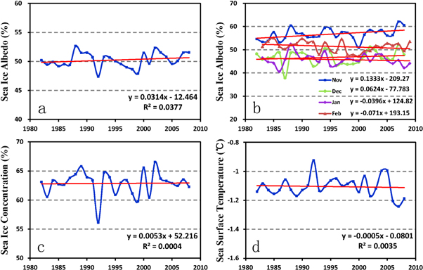
Figure 2. Regional Antarctic sea ice average spring–summer albedo (a), monthly (b), sea ice concentration (c), sea surface temperature (d), trends 1982–2009.
Download figure:
Standard image High-resolution image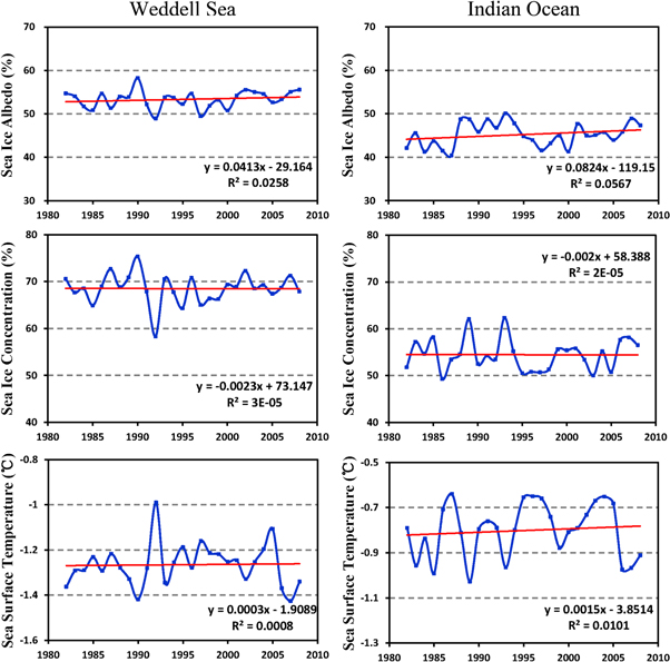
Figure 3. Average spring–summer Weddell Sea and Indian Ocean sector sea ice albedos, sea ice concentrations and sea surface temperatures from 1982 to 2009.
Download figure:
Standard image High-resolution image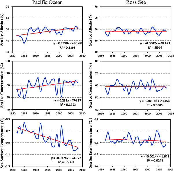
Figure 4. Averaged spring–summer Pacific Ocean and Ross Sea sector sea ice albedo, sea ice concentration and sea surface temperature from 1982 to 2009.
Download figure:
Standard image High-resolution image
Figure 5. Average spring–summer Bellingshausen–Amundsen Sea (BS) sector sea ice albedo, sea ice concentration and sea surface temperature from 1982 to 2009.
Download figure:
Standard image High-resolution imageWe found that the spring–summer averages for the sea ice zone albedo exhibited a slightly linear increasing trend throughout the time series (figure 2(a)), a linear trend slope of 0.314% per decade. For the five longitudinal sectors: the BS exhibited a negative trend of −1.617% per decade during the study period, whereas the RS albedo trend was near zero. The PO had the steepest positive trend of 2.599% per decade. The IO and the WS trends were 0.824% per decade and 0.413% per decade, respectively.
For the monthly albedo (figure 2(b)), the linear trend slope of 1.333% per decade in November was also distinctly higher than during the other three months (figure 2(b)). The mean albedo in November (56.69%) was also distinctly higher than the other three months (46.69% in December, 45.76% in January, and 51.40% in February). February is the last month of the summer, and the albedo in February was higher than in December and January for most years (figure 2(b)), because the sea ice in February consists mainly of multiyear ice, giving it a stable albedo. Once the surface ice melt begins, seasonal ice albedos are consistently less than the albedos for multiyear ice (Perovich and Polashenski 2012).
There was a low spring-summer average sea ice albedo in 1992 (figure 2(a)), which is consistent with the low SIC but in contrast to the high SST. This behaviour may be correlated with the snow-covered sea ice melting and wetting, thus lowering the albedo induced by the higher temperatures (Laine 2008). The summer (November, December, January) average Antarctic sea ice albedo from 1981 to 2000 increased at a rate of 0.1–3.7% per decade (Laine 2008); correspondingly, our results also appear to have an increasing trend of 0.3% per decade from 1982 to 2000, which is within Laine's range.
3.2. Spatial distribution
To illustrate the average spatial distribution of the albedo, SIC and SST, maps were prepared for the average spring–summer albedo, SIC and SST over the entire Antarctic sea ice region for the entire 28 years (figure 6). For each pixel, the final average was calculated by averaging the spring-summer four-month albedo for the entire 28 years.

Figure 6. Average spring–summer ice albedo 1982–2009 (a), Average spring–summer sea ice concentration 1982–2009 (b), Average spring–summer sea surface temperature 1982–2009 (c).
Download figure:
Standard image High-resolution imageThe sea ice albedo exhibited large spatial variation, ranging from 20% to 80% (figure 6(a)). The average value for the spring–summer sea ice albedo over the Antarctic sea ice region is approximately 50.24%. Spatially, the sea ice albedo was clearly higher off West Antarctica than in its eastern part. The high albedo values occurred on the continental coast and the WS, whereas the low values occurred on the outer edge of the sea ice, near the RS and the Amery Ice Shelf.
For each longitudinal sector, the average albedos, SIC, and SST with the corresponding trend, correlation coefficient, and significance level are shown in table 1. The highest sea ice albedo (53.33%) occurred in the WS, whereas the lowest sea ice albedo (45.22%) occurred in the IO, which may be associated with the formation of eddies and the upwelling of warm water (Zwally et al 2002). The average sea ice albedo in the BS was 51.34%; they were similar to those in the PO and the RS, at 48.07% and 48.18%, respectively.
Table 1. Average, trend and correlation coefficient of spring–summer sea ice albedos, sea ice concentrations and sea surface temperatures for Antarctica as a whole and for the five longitudinal sectors.
| Region | Trend (per decade) | Confidence level | Average | Correlation coefficient | Significance level |
|---|---|---|---|---|---|
| Sea ice albedo (%) | |||||
| Antarctic | 0.314 | / | 50.24 | / | / |
| WS | 0.413 | / | 53.33 | / | / |
| BS | −1.617 | 95.05 | 51.34 | / | / |
| IO | 0.824 | / | 45.22 | / | / |
| PO | 2.599 | 99.86 | 48.07 | / | / |
| RS | −0.002 | / | 48.18 | / | / |
| Sea ice concentration (%) | |||||
| Antarctic | 0.053 | / | 62.86 | 0.776 | 99 |
| WS | −0.023 | / | 68.51 | 0.712 | 99 |
| BS | −2.609 | 92.62 | 63.75 | 0.912 | 99 |
| IO | −0.020 | / | 54.47 | 0.737 | 99 |
| PO | 2.680 | 97.03 | 60.08 | 0.814 | 99 |
| RS | −0.097 | / | 59.07 | 0.859 | 99 |
| Sea surface temperature (°C) | |||||
| Antarctic | −0.005 | / | −1.11 | −0.590 | 99 |
| WS | 0.003 | / | −1.27 | −0.720 | 99 |
| BS | 0.081 | 98.11 | −1.04 | −0.843 | 99 |
| IO | 0.015 | / | −0.80 | −0.517 | 99 |
| PO | −0.128 | 99.98 | −0.81 | −0.686 | 99 |
| RS | −0.014 | / | −1.15 | −0.705 | 99 |
Note: '/' denotes insignificant correlation coefficient, and confidence level or significance level lower than 90%.
The average spring–summer sea ice albedos for each longitudinal sector have been compared with the ship-based field experiments from the Antarctic Sea Ice Processes and Climate (ASPeCt) dataset by Brandt et al (2005) (table 2). The ASPeCt albedo values are re-averaged from the spring and summer seasons for the same latitudinal ice areas (ice concentration at least 15%). The seasonal ASPeCt albedo averages include both ice and water. Moreover, the average ASPeCt albedos also have been weighted with the fractional coverage for each surface type (Brandt et al 2005). For comparison with the ASPeCt results, we recalculated the albedo averages for three months (November, December and January) from 1982 to 2000. As observed in table 2, our albedos are consistent with the ASPeCt results in the WS, RS and PS, and are close in the IO and PO.
Table 2. Average spring–summer sea ice albedos derived from the CLARA-A1-SAL and ASPeCt datasets for the five longitudinal sectors.
| Data/sectors | WS | IO | PO | RS | BS |
|---|---|---|---|---|---|
| ASPeCt | 53 | 48 | 40 | 48 | 52 |
| CLARA-A1-SAL | 51 | 43 | 46 | 49 | 52 |
Furthermore, to illustrate the sea ice albedo variations over 28 years, we averaged the spring–summer four-month albedos for each year, obtained their spatial distributions, and prepared maps of sea ice albedo from 1982 to 2008 (figure 7). The albedo patterns for the different years indicate little variability. In general, the albedo was between 20% and 80% in the Antarctic sea ice region; the variations in the sea ice extent were different for each year, and the highest albedo values were mostly found in the WS and on the continental coast, whereas the lowest albedo values (20–30%) occurred on the outer edge of the sea ice and in the RS, which is in agreement with figure 6(a).
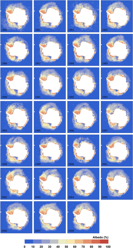
Figure 7. Spring–summer ice albedo 1982–2009.
Download figure:
Standard image High-resolution image3.3. Spatial distribution of the albedo trends
To gain a more illustrative and detailed view of the 28-year albedo trends, pixel-based spatial trend distribution maps were calculated for the entire Antarctic sea ice region (figure 8). The trends were calculated pixel-by-pixel using the least squares method for determining the best linear fit for the data. The trends were positive for most of the Antarctic sea ice regions (figure 8); they were strongly positive in some locations in the RS and WS (the WS had a trend of 0.413% per decade), as well as on the continental coast. Negative albedo trends can mostly be found in the western part of Antarctica, especially in the Bellingshausen–Amundsen Sea (with a negative trend of −1.617% per decade), and in part of the Ross Sea. However, the strongest local positive trend occurred in the east of the Weddell Sea and the Ross Sea, seaward from the Ross Ice Shelf. The Bellingshausen Sea and Amundsen Sea exhibited the strongest negative trends.

Figure 8. Change in the spring-summer ice surface albedo 1982–2009.
Download figure:
Standard image High-resolution image4. Discussion
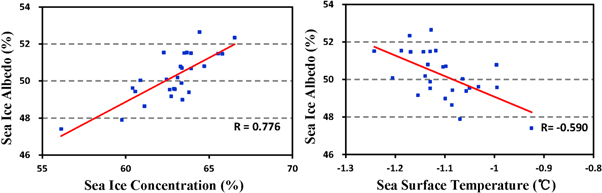
In general, the variations in sea ice concentration generally coincided with the albedo (figure 2(c)); the sea ice concentration in the Antarctic sea ice region showed a slight increasing trend similar to that of the albedo, but with a smaller trend. The linear slope trend was 0.053% per decade. The correlation coefficient of the SIC and sea ice albedo was 0.7760 (with a significance level of 99%) (figure 9). The SIC in 1992 exhibited a low value (figure 2(c)), which corresponded with the albedo.
Figure 9. The relationships between the spring–summer sea ice albedos and the sea ice concentrations and sea surface temperatures.
Download figure:
Standard image High-resolution image
In the five longitudinal sectors, the BS has the steepest negative trend of −2.609% per decade during the study period; the PO had the steepest positive trend of 2.68% per decade, whereas the RS, IO and WS had SIC trends near zero. The SIC and sea ice albedo in all five longitudinal sectors were well correlated, and all of their significance levels were 99% (table 1).
The spatial variations of the SIC were between 15% and 90% (figure 6(b)), and the mean was 62.86%. The higher surface albedo was due to a higher sea ice concentration. A high concentration of sea ice was also found on the continental coast and in the WS, whereas low concentrations of sea ice can be observed on the outer edge of the sea ice, the RS and near the Amery Ice Shelf; these results coincide with the albedo. This may be connected with sea ice melting and coverage decreasing. As we know, the albedo of sea ice is larger than open water. Therefore, the sea ice melting leads to a lower albedo, induced by higher temperatures. The highest values of both the sea ice albedo (53.33%) and the SIC (68.51%) occurred in the WS, whereas the lowest values of both the sea ice albedo (45.22%) and the SIC (54.47%) occurred in the IO.
The SST narrowly fluctuated: its trend was not significant, the linear trend slope was −0.005 °C per decade, and the mean was −1.105 °C from 1982 to 2009. The albedo was significantly negatively correlated with the SST (figure 2(d)), and the coefficient was −0.58 (at 99% significance level) (figure 9). The SST in 1992 had an extremely high value, which resulted in a decrease in the albedo and the SIC.
For the five longitudinal sectors, the PO had the steepest negative trend of −0.13 °C per decade. This means that the temperature has declined over the past decades. The temperature decline has resulted in a significant increase in the area of snow covered sea ice and sea ice formation, leading to an increase in the surface albedo (Screen and Simmonds 2012). The BS had the positive trend of 0.081 °C per decade. The increasing temperature over the BS has led to the increasing proportion of non-frozen precipitation and then reduces the albedo in this region (Kirchgäßner 2011). The SST trends in the other three longitudinal sectors were not significant and were near zero. However, the albedo and the SST in all five longitudinal sectors were significantly negatively correlated (at 99% significance level) (table 1).
Spatially, the SST corresponds well with the albedo; the higher surface albedos follow the lower temperature patterns. Because the albedo is strongly controlled by the ice thickness and snow cover, and the temperature is a proxy for these parameters. Thick ice with snow cover has a lower surface temperature and has, in general, a higher albedo, whereas thin sea ice, without snow cover, shows a relatively warm temperature and a low albedo (Weiss et al 2012). Thus, the spatial distribution of the SST was in contrast to the sea ice albedo; the SST gradually decreased as the latitude increased (figure 6(c)). The highest values in the SST occurred on the outer edges of the sea ice, whereas the lowest values existed in the RS and WS, as well as on the continental coast. The highest sea ice albedos (53.33%) and the lowest SST (−1.27 °C) occurred in the WS, whereas the lowest sea ice albedos (45.22%) and highest SST (−0.8 °C) occurred in the IO.
In the five longitudinal sectors, the highest sea ice albedos corresponded well with the highest SICs and the lowest SSTs in the WS and IO. The highest sea ice albedos (53.33%), SIC (68.51%) and lowest SST (−1.27 °C) occurred in the WS, whereas the lowest sea ice albedos (45.22%), SIC (54.47%) and highest SST (−0.8) occurred in the IO.
5. Conclusions
Over the entire Antarctic sea ice region, the albedo, SIC and SST all exhibited substantial annual variabilities from 1982 to 2009. The sea ice albedo slightly increased at a rate of 0.314% per decade. The average value for the spring-summer sea ice albedo was 50.24%. The average albedo in the western Antarctic sea ice region was higher than in the east. The highest albedo values are mainly found on the continental coast and in the WS; however, the lowest albedo values existed on the outer edge of the sea ice in the RS and the Amery Ice Shelf.
For each longitudinal sector, the BS had a negative trend of −1.617% per decade during the study period, whereas the albedo trend in the RS was near zero. The PO sector had the steepest positive trend of 2.599% per decade, and the IO sector and the WS had trends of 0.824% per decade and 0.413% per decade, respectively. The highest sea ice albedos (53.33%) occurred in the WS, whereas the lowest sea ice albedos (45.22%) occurred in the IO. The average albedo in the BS was 51.34%, and in the PO and RS, they were similar, at 48.07% and 48.18%, respectively.
The albedo was significantly positively correlated with the SIC and was significantly negatively correlated with the SST, both at a 99% significance level; these scenarios were true for all five longitudinal sectors. Spatially, the higher surface albedos follow the higher sea ice concentrations and the lower temperature patterns. The highest sea ice albedo and SIC and lowest SST occurred in the WS sector, whereas the lowest sea ice albedos, SIC and highest SST occurred in the IO sector.
Several factors affected the black-sky albedo in the Antarctic sea ice region. Antarctic sea ice is always covered by snow; therefore, the snow depth, grain size and wetness play an important role in the albedo. For the snow-free sea ice albedo, the sea ice thickness is an important factor in the albedo, especially for thin ice (0–30 cm) (Lindsay 2001). In the thin ice regions, ice thinning or growth can be a significant cause of changes in albedo. The Antarctic sea ice regions experience flooding by seawater and wave overwashing (Massom et al 2001), which lower the albedo by removing the snow cover and wetting the snow. Furthermore, snowfall, drift snow transport and snow metamorphism also affect the sea ice albedo.
Removing points or changing the beginning or ending time of a time series can change the significance of a linear trend, or even completely change the sign of the slope (Watkins and Simmonds 2000, Laine 2008). Any extrapolation of the trend lines beyond the 28-year study period is not scientifically valid. In the future, more in situ SST and albedo data are necessary to validate the satellite retrieval results. Combined satellite and station data can provide reliable tools for evaluating the variability of the sea ice in the Antarctic regions.
Acknowledgments
The authors would like to thank the CM SAF team at the Deutscher Wetterdienst for processing the CLARA-A1-SAL dataset. We thank the National Snow and Ice Data Center for the sea-ice concentration data. We thank the NOAA Earth Systems Research Laboratory for providing the National Centre for Environmental Prediction-Department of Energy Reanalysis 2 data. The NOAA_OI_SST_V2 data are provided by the NOAA/OAR/ESRL PSD, Boulder, Colorado, USA, from their Web site at http://www.esrl.noaa.gov/psd/. The authors would like to thank the above data providers. This work is supported by the Programme for National Nature Science Foundation of China (No. 41371391), the Programme for Chinese National Antarctic and Arctic Research Expedition (CHINARE2015-02-02), the Programme for Foreign Cooperation of Chinese Arctic and Antarctic Administration (No. IC201301), and the Programme for the Specialized Research Fund for the Doctoral Program of Higher Education of China (No. 20120091110017).