

Abstract
To understand the governing mechanisms of bio-inspired swimming has always been challenging due to intense interactions between flexible bodies of natural aquatic species and water around them. Advanced modal decomposition techniques provide us with tools to develop more in-depth understating about these complex dynamical systems. In this paper, we employ proper orthogonal decomposition (POD) and dynamic mode decomposition (DMD) techniques to extract energetically strongest spatio-temporal orthonormal components of complex kinematics of a Crevalle jack (Caranx hippos) fish. Then, we present a computational framework for handling fluid–structure interaction related problems in order to investigate their contributions towards the overall dynamics of highly nonlinear systems. We find that the undulating motion of this fish can be described by only two standing-wave like spatially orthonormal modes. Constructing the data set from our numerical simulations for flows over the membranous caudal fin of the jack fish, our modal analyses reveal that only the first few modes receive energy from both the fluid and structure, but the contribution of the structure in the remaining modes is minimal. For the viscous and transitional flow conditions considered here, both spatially and temporally orthonormal modes show strikingly similar coherent flow structures. Our investigations are expected to assist in developing data-driven reduced-order mathematical models to examine the dynamics of bio-inspired swimming robots and develop new and effective control strategies to bring their performance closer to real fish species.
Export citation and abstract BibTeX RIS
1. Introduction
For the last two decades, scientific community has made a lot of progress to understand the natural aquatic locomotion of numerous species that can enable them to utilize the discovered hydrodynamic mechanisms to propose efficient and maneuverable designs for bio-inspired underwater vehicles (Fish 2020). In spite of this substantial amount of efforts previously, there exists a huge gap to design effective flow control strategies for these robotic devices. A major difficulty in this pursuit relates to the involvement of uncertain real conditions in large water reservoirs, such as oceans and rivers, to be faced by swimming robots and the prediction of their dynamical states impacted by numerous physical factors. In this context, data-driven techniques come up as great candidates for predicting complex nonlinear flow dynamics and tuning the kinematics of the flexible body-structures of fish-like robots (Brunton et al 2020, Verma et al 2018) to obtain desired performance levels. This scenario has also raised the requirement of developing effective reduced- or low-order mathematical models to describe the mechanics of these engineering systems that would open up new horizons to apply machine learning or deep learning control techniques in this field. For the dimensionality reduction, advanced modal decomposition techniques, such as proper orthogonal decomposition (POD), dynamic mode decomposition (DMD) and their variants (Rowley and Dawson 2017) provide great tools to extract primary features of nonlinear dynamical systems without really solving the governing equations. Previously, several people reported their efforts to utilize these techniques to understand underlying hydrodynamic mechanisms for bio-inspired flows. Ting and Yang (2009) used singular-value decomposition (SVD) method to extract key flow features in the two-dimensional wake of a fish. Some other studies (Liang and Dong 2015, Li et al 2016, Li et al 2017, Han et al 2017) presented the utility of POD technique based on a traditional eigenvalue decomposition analysis for flows around flapping wings and plates. These investigations also proposed the concept of virtual force to classify the modes to find their contributions in the production of lift and thrust forces.
There is another interesting way of investigating the effects of dominant structural modes to quantify their relative contributions in the production of total hydrodynamic forces on bio-inspired structures during their steady swimming. For example, Bozkurttas et al (2009) utilized the SVD formulation to determine that only three structural POD modes were sufficient to model the complex dynamics of a flexible pectoral fin of a bluegill sunfish. They concluded that the kinematics reconstructed by the mean and three oscillatory POD modes was able to produce 92% of the thrust force generated by the full-order kinematics of the pectoral fin. Ren and Dong (2016) used a similar methodology to decompose the morphing wing kinematics of a hovering dragonfly to examine the effects of POD modes on its aerodynamic performance.
Besides, there were a few recent efforts to break down the travelling-wave like motion of different carangiform swimmers (Feeny and Feeny 2013, Tanha 2018). Feeny and Feeny (2013) considered the transverse kinematics of a whiting and carried out complex modal analysis. They found that a single complex mode was enough to represent the transverse wavy motion of the fish. In this formulation, this complex mode had two components out of which the real one showed a standing wave and the imaginary part represented a traveling wave like structure. Following a similar approach, Tanha (2018) employed the modal information to approximate important kinematic parameters, such as oscillation amplitudes and phases and their dependence on time and spatial location on fish bodies. However, the low-dimensional analyses conducted in the afore-mentioned studies were limited to the kinematics of flexible structures. The connections between dominant kinematic modes and primary flow features of complex fluid–structure interaction-based systems are still elusive.
Recent advancements in the field of modal analysis to characterize complex dynamical systems have opened doors to analyze the underlying mechanics of bio-inspired systems. A very significant element of such systems is the nonlinear interaction between the involving fluids and structures. Although a common approach is to segregate the flow field information from the overall system and examine its dynamical properties, yet it would be very informative to incorporate the structural kinematics into these mathematical and computational frameworks to determine the levels of coupling between the fluid and structures. This approach will also enable us to segregate contributions of the fluid and structures towards the dynamics of the overall system. The only effort in this account found in literature was done by Goza A and Colonius T (2018) in which they considered a two-dimensional flow field around a flapping flag and analyzed its limit-cycle and chaotic dynamics.
In our current study, we present a computational framework to look for energetically strong modal decompositions for three-dimensional dynamical systems involving prescribed fluid–boundary interaction. We employ the physiology of a jack fish the motion of which has been recorded live by a high-speed photogrammetry system. First, utilizing POD on the data set of its structural configurations enables us to propose a low-dimensional description of its complex flexible body kinematics. Next, we use POD and DMD approaches to investigate fluid–structure interactive mechanics and explain formation and production of primary coherent fluid structures for two Reynolds numbers: 500 and 4000. We perform the modal analyses in a prescribed fluid–boundary interaction framework for the flow over the caudal fin only due to the following two reasons, (1) the inclusion of a thick body structure in this computational framework will lead to spurious flow oscillations around and inside the body Goza A and Colonius T (2018) Menon K and Mittal R (2020), and (2) the caudal fin is the primary thrust producing component for a jack fish as also explained by Liu et al (2017).
The manuscript is organized as follows. Section 2 explains our computational methodology to perform numerical simulations using a sharp-interface immersed boundary method-based solver. It also provides details for our approach to conduct modal analyses of the kinematics of a jack fish and the prescribed fluid–fin interaction-based system composed of the membranous caudal fin and the vortical flow field around it. Next, we present our analyses and findings about the low-dimensional description of this highly nonlinear system using POD and DMD in section 3. Finally, we summarize and conclude our work in section 4.
2. Computational methodology
In this section, we elucidate our computational methodology to handle the reconstruction of the physiological model of a jack fish and its kinematics. We also explain the numerical methodology based on a sharp interface immersed-boundary method to perform numerical simulations for flows over the caudal fin at Reynolds numbers (Re = U ∞ L / ν ) 500 and 4000. Here, ν indicates kinematic viscosity of the fluid, U ∞ stands for free-stream velocity, and L is the entire body-length of the jack fish. Moreover, we summarize POD and DMD techniques and illustrate our strategy to set up snapshot data matrices for their further processing in order to extract the most dominant modal characteristics for the kinematics of a jack fish and the prescribed fluid–boundary interaction based system of its caudal fin. Due to capturing the real fin motion and its incorporation in our computational solver, we argue that this whole system forms the basis of our claim about the interaction between the fluid flow and the structural oscillations in our present study. As explained in subsequent sections, the consistency in finding the same Strouhal number for all the swimming speeds of the jack fish also supports this argument.
To illustrate more on this aspect in our present work, we use the real fish kinematics recorded and reconstructed through high-speed cameras. This same kinematics is further utilized in our IBM-based CFD solver. This integrated experimental-numerical approach allows us to analyze hydrodynamics and resultant wake features produced by real fish motion. Because the live recording effectively captures the flexible body dynamics of the membranous caudal fin, we consider it a fluid–fin interaction system where the structural response has already been taken care of by the high-speed photogrammetry technique. We obtain the formation and dynamics of coherent flow structures through our CFD solver. Thus, this whole approach justifies the use of the term prescribed fluid–boundary interaction. As far the computational approach is concerned, our current system seems to present more like one-way FSI (from structure to fluid), but the integration of experimentally determined real kinematics gives us the actual structural response thus taking care of the feedback of the fluid to affect the structural response. It is important to mention that the present kinematics was found to be statistically robust for a wide range of swimming speeds of jack fish (Liu et al 2017).
2.1. Jack fish physiological model and kinematics
To reconstruct the geometry of a jack fish and its kinematics, we employ the data recorded and reported previously by (Liu et al 2017) to investigate the body–fin and fin–fin interaction during its steady swimming. Although the procedure to capture the fish motion and its physiology along with the statistical details has been covered in reference (Liu et al 2017), we present its salient points here as well for the sake of completeness. The current model is of Crevalle jack (Caranx hippos) which is classified as a carangiform swimmer. Out of total 12 individuals of this class of fish with a mean total length L = 0.338 m and swimming at 1L s−1 to 4L s−1. It is important to highlight that their body kinematics did not change much with the increasing swimming speed. The currently used kinematic data was adopted from an individual fish having L = 0.31 m and swimming at 2L s−1. The total height and width, normalized by L, of this fish are 0.286 and 0.144, respectively. The area, normalized by L2, of the caudal fin is 0.023 and its normalized length is 0.244. The normalized height and length of the caudal fin are 0.315 and 0.244, respectively.
In this study, we consider the trunk and caudal fin only because these two components primarily contribute towards the kinematics and functionality of a fish. Its trunk is modeled as a solid body with a closed surface and the caudal fin is a membrane with zero thickness. Each surface is, then, represented by triangular mesh where the main body is composed of 11 358 nodes and 22 712 elements. The surface of the caudal fin has 1369 nodes and 2560 elements (see figure 1(c)). The measured wavelength from the midline profiles is approximately 1.05L which is a characteristic of the carangiform swimming mode. The measured Strouhal number (St) for these recordings remain 0.30, where St = 2AfE/U with fE being the excitation/flapping frequency of the caudal fin, A as the maximum one-sided oscillation amplitude of the caudal fin, and U as the swimming speed.
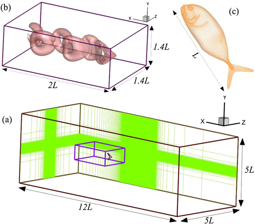
Figure 1. (a) Virtual tunnel for simulating flows over the caudal fin of a jack fish with its dimensions where the inner box shows the domain to extract data for modal decompositions, (b) a zoomed-in view of the inner domain covering the caudal fin and coherent flow structures in its wake, and (c) jack fish body and caudal fin covered with a mesh to indicate the marker points to track their motion.
Download figure:
Standard image High-resolution image2.2. Numerical solver
We perform three dimensional (3D) numerical simulations for flows over the oscillating caudal fin; a membranous structure, at Re = 500 and 4000. Following non-dimensional forms of the continuity and incompressible Navier–Stokes equations constitute the mathematical model for the fluid flow:
where the indices  , xi
shows Cartesian directions, the ui
denotes the Cartesian components of the fluid velocity, p is the pressure, and Re represents the Reynolds number.
, xi
shows Cartesian directions, the ui
denotes the Cartesian components of the fluid velocity, p is the pressure, and Re represents the Reynolds number.
We solve the described governing model for fluid flow using a Cartesian grid-based sharp-interface immersed boundary method (Mittal et al 2008) where the spatial terms are discretized using a second-order central difference scheme and a fractional-step method is employed for time marching. This makes our solutions second-order accurate in both time and space. We utilize the Adams–Bashforth and implicit Crank–Nicolson schemes for the respective numerical approximations of convective and diffusive terms. The prescribed wavy kinematics is enforced as a boundary condition for the swimmers. We impose such conditions on immersed bodies through a ghost-cell procedure (Mittal et al 2008) that is suitable for both rigid and membranous body-structures. Further details of this solver and its employment to solve numerous bio-inspired fluid flow problems are available in references (Liu et al 2017, Wang et al 2019, Han et al 2020, Wang et al 2020).
Next, we employ Dirichlet boundary conditions for flow velocities on all sides except the left one where Neumann conditions are used at the outflow boundary (see figure 1(a)). The slices on the back and left boundaries show the regions with high mesh density in order to adequately resolve the flow features around the structure and its wake. The rectangular box in figure 1(b), encompassing the swimmer's body, shows the region of which we extract the data to perform our modal analysis. We use a mesh size  for the complete flow domain, while the extracted domain for our further analysis has a mesh size
  . For the mesh independent study, the readers are referred to the reference (Liu et al
2017). It means that the total number of nodes in the entire flow domain and its extracted part are 7.99 million and 4.40 million, respectively.
. For the mesh independent study, the readers are referred to the reference (Liu et al
2017). It means that the total number of nodes in the entire flow domain and its extracted part are 7.99 million and 4.40 million, respectively.
2.3. Proper orthogonal decomposition
Proper orthogonal decomposition technique provides us with a data analysis method focusing on extracting energetically ranked modes to propose relevant mathematical models in order to describe the system dynamics with reduced dimensionality (Akhtar et al 2009). This strategy gives us optimal and orthonormal spatio-temporal modes of a dataset. POD modes and their associated useful information can be obtained by employing either eigenvalue decomposition of the covariance matrix of a dataset or by performing singular value decomposition (SVD) of the data matrix. In this data matrix, information about the states of a dynamical system is stored and arranged in particular patterns to further process it by utilizing these techniques.
In our present study, we perform the POD analysis through the SVD technique. The main focus here is to use modal decomposition methods for two purposes: (1) to extract significantly reduced-dimensional information for the complex wavy kinematics of a jack fish and (2) to propose a computational framework in order to perform modal analyses of fluid–structure interaction based systems and capture the most relevant information about both the structural motion and flow field. It is customary to exclude the time-averaged profiles of a dataset before applying POD. This practice makes it equivalent to principal component analysis (PCA) in the fields of imaging, video processing, and computer graphics (Perlibakas 2004). To decompose the fish kinematics into its primary POD modes, we construct the following snapshot data matrix:
where ξ, η, and ζ denote the displacements of each nodal point on the surface of the fish in x, y, and z directions, respectively. The subscripts B and CF indicate the information belonging to the main body (trunk) and caudal fin, respectively. This snapshot matrix contains the motion information of 48 time instants spanning one complete oscillation cycle of the jack fish. The SVD is formulated as:

where
U
is a unitary matrix containing left eigenvectors of the snapshot data matrix
X
S
, Σ is a diagonal matrix with positive numbered entries σi
termed as singular values and arranged in the descending order, i.e., σ1 ⩾ σ2 ⩾ σ3 ... . ⩾ σN
, and
V
is another unitary matrix. The eigenvalues (λ) can be computed by squaring σ values. It is important to highlight that the columns of
U
matrix give us the spatial distribution of POD modes, whereas
V
contains the information about the temporal variations in these modes. Each column of the
V
matrix provides us the temporal coefficients (α) of the POD modes. To connect it with the traditional eigenvalue decomposition,
U
and
V
are the eigenvectors of covariance matrices  and
and  , respectively. Conventionally, the sizes of
U
, Σ, and
V
matrices are (3NB + 3NCF) × (3NB + 3NCF), (3NB + 3NCF) × NT, and NT × NT, respectively. However, performing the 'economy' SVD in MATLAB enables us to obtain and process
U
and Σ matrices with their respective sizes of (3NB + 3NCF) × NT and NT × NT which reduces the computational burden to a large extent and prevents us from facing out-of-memory problems during numerical processing.
, respectively. Conventionally, the sizes of
U
, Σ, and
V
matrices are (3NB + 3NCF) × (3NB + 3NCF), (3NB + 3NCF) × NT, and NT × NT, respectively. However, performing the 'economy' SVD in MATLAB enables us to obtain and process
U
and Σ matrices with their respective sizes of (3NB + 3NCF) × NT and NT × NT which reduces the computational burden to a large extent and prevents us from facing out-of-memory problems during numerical processing.
A reduced-order reconstruction for the system's kinematics or dynamics can be attained by using U , Σ, and V matrices in the basic formulation of SVD. To obtain the temporal behavior (video) of a particular ith POD mode, we can make all the entries zero except its particular singular value σi in the Σ matrix. Thus, the mathematical form for this concept is;

In order to utilize this technique for a system based on fluid–structure interaction, we construct our snapshot matrix using the entries pertaining to the dynamical states of both the structure, the caudal fin in this case, and fluid flow in the following form:
Here, u, v, and w are the Cartesian components of the fluid velocity, and each column represents a snapshot of the FSI system at one time instant.
2.4. Dynamic mode decomposition
Dynamic mode decomposition (DMD) provides a computational framework to extract a primary low-order description of a data set through its orthonormal modes in a temporal sense. The DMD modes are also approximations of the Koopman operator which is a linear infinite dimensional operator representing a nonlinear dynamical system onto the Hilbert space of the functions and states under consideration (Kutz et al
2016). It enables us to build a linear description of a complex dynamical system without losing its nonlinear characteristics. The sole idea is to construct a formulation of a dynamical system
x
(t) such that  ,
,  , and so on. In other words, we have
  . This method computes DMD modes for the matrix A by minimizing ||
 ||, where the subscripts k and k − 1 are some time-instants.
For this purpose, we distribute the original snapshot data matrix
X
into two submatrices
X
1 and
X
2, where ![${\boldsymbol{X}}_{1}=\left[{X}^{{t}_{1}}{X}^{{t}_{2}}\cdots {X}^{{t}_{N-1}}\right]$](https://content.cld.iop.org/journals/1748-3190/16/1/016018/revision4/bbabc294ieqn10.gif) and
and ![${\boldsymbol{X}}_{2}=\left[{X}^{{t}_{2}}{X}^{{t}_{3}}\cdots {X}^{{t}_{N}}\right]$](https://content.cld.iop.org/journals/1748-3190/16/1/016018/revision4/bbabc294ieqn11.gif) . For further details on the algorithm, the readers are referred to references (Rowley et al
2009, Schmid 2010, Schmid 2011, Kutz et al
2016). In order to exploit the underlying data-driven technique, this algorithm indirectly solves for the DMD modes Φ of A matrix. To reduce the computational cost incurred due to the large amount of data set, we, first, perform the POD and truncate the lowest energy-ranked modes to include the most relevant information in the DMD computations. The real and imaginary parts of the corresponding DMD eigenvalues; λr and λi, respectively, denote the growth rate and frequency of DMD modes. Next, the associated angular frequencies having units rad/ sec is computed by
. For further details on the algorithm, the readers are referred to references (Rowley et al
2009, Schmid 2010, Schmid 2011, Kutz et al
2016). In order to exploit the underlying data-driven technique, this algorithm indirectly solves for the DMD modes Φ of A matrix. To reduce the computational cost incurred due to the large amount of data set, we, first, perform the POD and truncate the lowest energy-ranked modes to include the most relevant information in the DMD computations. The real and imaginary parts of the corresponding DMD eigenvalues; λr and λi, respectively, denote the growth rate and frequency of DMD modes. Next, the associated angular frequencies having units rad/ sec is computed by  , and its further division by 2π gives us the linear frequency in Hertz. Here, Δt is the sampling time to obtain the snapshot data matrix. We obtain the approximate solution for the next time instants using the following form:
where bj is the initial amplitude, serving as the initial condition as well, of the jth mode.
3. Results & discussion
Before discussing the modal analysis for the kinematics of a jack fish and the flow fields around its oscillating caudal fin at different Reynolds numbers, it is important to explain the temporal character and the frequency components of hydrodynamic forces on the caudal fin. For this purpose, we define the nondimensional hydrodynamic force components as C = F /0.5 ρU 2 A CF , where A CF is the area of the caudal fin. Subscripts of C represents the direction of each force component. Figure 2 presents temporal variations of the horizontal (drag/thrust) and lateral forces. We find that C X = C D tends to change its instantaneous magnitude levels with a change in Re, and there exists a small change in its phase as well. Nonetheless, C Z shows almost similar patterns for both Reynolds numbers though higher Re causes a smaller increase in its positive and negative peak values. The spectral decompositions of horizontal, lateral, and sideways forces in figure 3 reveal that the excitation frequency of the caudal fin f E is the most dominant frequency in the Fourier spectra of C Z . However, both C D and C Y possess the frequency 2 f E as the strongest one with smaller contributions from f E and its higher harmonics. These observations are consistent with those from flows over cylinders (Imtiaz and Akhtar 2017) and flapping wings (Khalid et al 2015, Khalid et al 2018, Liang and Dong 2015).
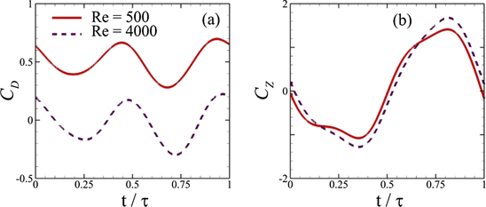
Figure 2. Time histories of hydrodynamic force coefficients in the horizontal and lateral directions.
Download figure:
Standard image High-resolution image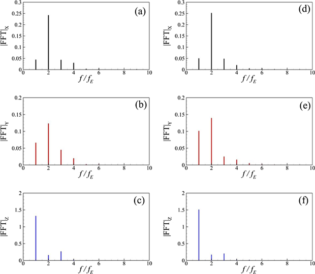
Figure 3. Fourier spectra of hydrodynamic force coefficients along the Cartesian axes, (a) and (d) drag/thrust force, (b) and (e) vertical force, and (c) and (f) lateral force, where the left and right columns show data for Re = 500 and 4000, respectively.
Download figure:
Standard image High-resolution image3.1. Fish kinematics
Due to the flexibility of their bodies, different species of fishes perform complex wavy motions, usually known as undulation composed of travelling waves along their bodies [see supplementary movie 1 (https://stacks.iop.org/BB/16/016018/mmedia)]. Using the POD technique, we decompose its full-order kinematics into spatially orthonormal modes. Figure 4 shows the POD eigenvalues normalized by their summation that represent the corresponding energy levels of each mode. It is evident that the first POD mode constitutes approximately 79% of the energy, whereas the second POD mode has more than 20% energy. All the other modes carry almost zero energy levels. Thus, seemingly complex carangiform motion mainly comprises of only two primary modes.
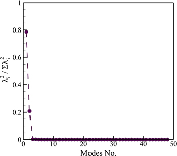
Figure 4. Energy levels of POD modes of a jack fish kinematics.
Download figure:
Standard image High-resolution imageTo illustrate it further, we represent the instantaneous positioning of the fish trunk during its one oscillation cycle for the first two modes in figure 5 (see supplementary movies 2–4). In both the modal configurations, the posterior part of the body shows a greater amount of displacement from its equilibrium position that is a characteristic feature of carangiform and sub-carangiform swimming patterns. The first POD mode shows a standing wave like structure where the nodes and antinodes are evidently visible. The first node is located at 17% of the total body-length, whereas the second one is positioned at 0.59L. The orientations of the trunk section of the second POD mode shows that the main body pitches about the y-axis passing through a point at 0.34L. However, these configurations combined with those of the caudal fins give another standing wave along its length, where the first and second nodes are located at  and 0.84L. Moreover, looking at the caudal fin alone in its POD modes 2, we observe its pitching motion about the mid-points of its dorsal and ventral peripheries. Its formation in POD mode 1 exhibits a flapping motion; a combination of heaving and pitching. It is interesting to notice that both the POD modes demonstrate left–right asymmetry for the trunk section and the caudal fin. We observe prominent dorsal–ventral asymmetry for the caudal fin by comparing its orientations. It appears that the pitching angle of the ventral side of the caudal fin is lesser than that of its dorsal side. A careful look at the instantaneous configurations in figures 5(a) and (b) reveals that there exists a phase angle of π/2 between the two POD modes. Hence, the entire undulatory kinematics of a jack fish comes out to be the summation of its mean position and two standing waves moving with a phase of π/2.
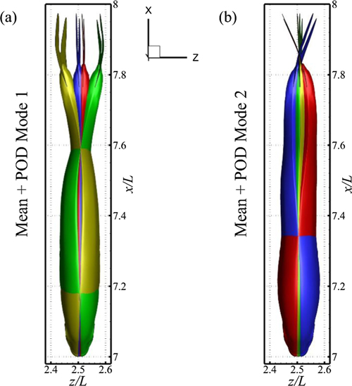
Figure 5. Modal configurations of the trunk and caudal fin of a jack fish where color coding is used to distinguish between the instantaneous positions: red ( ), green (
 ), blue (
 ), and yellow (
 ).
).
Download figure:
Standard image High-resolution image3.2. Flow fields analysis
Here, we perform numerical simulations for flows over the caudal fin of a jack fish at two Reynolds numbers: 500 and 4000. These two flow conditions are representatives of viscous (Re ∼ 102) and transition (Re ∼ 103) flow regimes.
We present time-averaged flow fields in the wake of the caudal fin for both Reynolds numbers being considered for this study in figure 6. As observed in the top-most row, there exist four distinct vortex tubes at Re = 500 and six tubal structures are present at Re = 4000. It seems that an increase in Re breaks the two vortex tubes on the dorsal side of the caudal fin, and the remaining two on the ventral side remain intact with a few signs of disruptions as they get developed in the downstream direction. Here, four tubes are elongated, and the other two new tubes developed due to the higher Re remain shorter. Because these structures traverse downstream at an inclination, they tend to diverge from each other. To elucidate the symmetry features of these flow fields, we plot contours of the Cartesian components of vorticity; ωx , ωy , and ωz , on surfaces normal to their corresponding axes. For Re = 500, the x-component of vorticity (ωx ) shows four distinct coherent structures reminiscent of the formation of four vortex tubes in the wake of the caudal fin. It is clear that ωx demonstrates symmetry about the diagonal axis joining the two corners of the plane as drawn in figure 6(b).
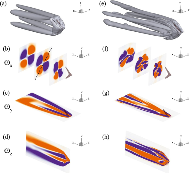
Figure 6. Mean flow fields and their symmetry properties using Cartesian components of vorticity where the left (a)–(d) and right (e)–(h) columns show data for Re = 500 and 4000. The plots in the 1st row are drawn using Q-criterion. The 2nd, 3rd, and 4th rows represent data on the corresponding planes for ωx , ωy , and ωz , respectively.
Download figure:
Standard image High-resolution imageIn such a problem, there may exist four independent reflection symmetries, denoted as SX , SY , SZ , and SD with respect to the x, y, z -axes and a diagonal axis y + z. We use the following forms to mathematically define these symmetry characteristics.
Employing these terms, ω x holds S D symmetry for the mean flow field at Re = 500, but we do not find any symmetry for ω x at Re = 4000 with the existence of a few coherent structures here. Observing the contours of ω y and ω z on xz and xy planes, respectively, reveals the formation of four shear layers for the lower Re and six shear layers at the higher Re. Considering the three contour plots in figure 6(f), we come to know that the development of distinct coherent vortical structures should be carefully analyzed for complex flows because their orientations and characteristics may change as we move downstream. It may also result in the switching of symmetric and asymmetric flow features to be explained later in the study.
Performing POD for the snapshot data containing information for both the fluid and structural motion provides us with the knowledge about how much contribution each POD mode would have in this complex dynamical system. We present the energy levels of POD modes for our full FSI system through the squared and normalized eigenvalues in figure 7 for Re = 500 and 4000. For the viscous flow regime, the first two modes contribute 36.5% and 33.6% energy to the overall system dynamics. The remaining modes exist in pairs due to periodic oscillations of both the caudal fin and vortices in the wake. The same phenomenon was observed for flows over circular cylinders at very low Re previously (Taira et al 2020). Here, the first four modes have more than 85% of the total energy of this dynamical system. Analyzing the data in figure 7(b) for Re = 4000 also reveals similar trends. Here, the POD modes 1 and 2, respectively, have 32.7% and 29.4% of the total energy. As expected, we need to include six POD modes to capture around 85% of the energy due to a smaller effect of viscosity under these conditions. Even though the viscous action is at a reduced level for the higher Re, we observe the formation of pairs reflecting order to a large extent. Nevertheless, it is interesting to note that the structural elements in our data would only contribute to the first two POD modes for both the flow conditions because we do not see substantial oscillations of the caudal fin in the higher POD modes (see supplementary movies 5 and 6). It means that the caudal fin as the oscillating structure only contributes towards the development of the first two POD modes, and the oscillatory patterns in the higher POD modes find their origin in the fluid dynamics only.
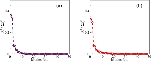
Figure 7. Squared eigenvalues normalized by their summation for (a) Re = 500 and (b) 4000.
Download figure:
Standard image High-resolution imageNow, we present the POD modes of our FSI system at Re = 500 and 4000 in figures 8(a)–(c) and 9(a)–(c), respectively. For the lower Reynolds number conditions, the flow structures tend to form a shape of a 'headless panda' (quadfurcated shape) with four small arms extended in the downstream direction. Nevertheless, these arms like structures vanish in the higher POD modes and we see only planar structures aligned closely with each other. For Re = 4000, these features adopt hairpin-like shapes as presented in figure 9, but these flow features lose their distinct shape when we see the higher POD modes here although the formation and presence of coherent flow structures are evident there as well.
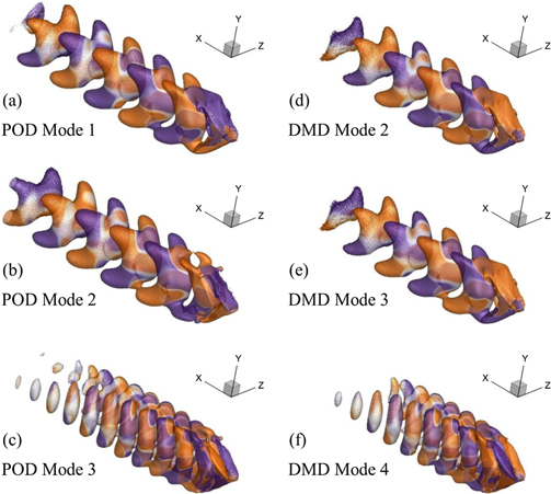
Figure 8. Most dominant oscillatory POD and DMD modes for our FSI system working at Re = 500.
Download figure:
Standard image High-resolution image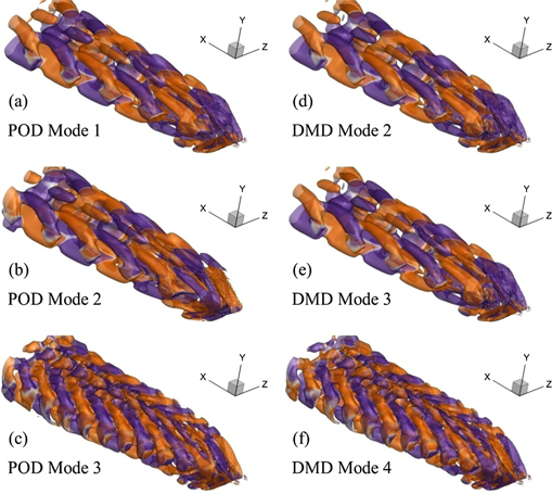
Figure 9. Most dominant oscillatory POD and DMD modes for our FSI system working at Re = 4000.
Download figure:
Standard image High-resolution imageIn table 1, we provide symmetry characteristics of the first 8 POD modes for each flow condition. We discover that the lateral component of vorticity (ωz ) always shows asymmetry, whereas the other two components; ωx and ωy , show variations in their properties. It is also important to note that each pair of POD modes possesses similar characteristics despite the complex motion of the caudal fin and the vortex patterns in its wake. While moving xy, yz, and xz planes along their corresponding normal axes, we find that the symmetry properties of these dynamical systems do not remain consistent throughout the wake. Instead, they may momentarily switch their states with some asymmetric patterns to regain symmetry afterwards. We explain those conditions in table 1. An important feature of our analysis is that, for a few significant POD modes at Re = 4000, ωy exhibits symmetric coherent patterns about the axis parallel to the xz-plane and the one cutting it into two halves only when the plane lies in the middle of the domain. Thus, it is of utmost importance that extreme care should be taken while performing such analyses using experimental techniques where middle planes are usually selected to find the traits of coherent structures. Another salient observation is the increasing number of asymmetric flow patterns of the POD modes at the higher Re.
Table 1. Symmetry properties of mean and POD modes of our FSI systems.
| Reynolds No. | POD mode number |

|

|

|
|---|---|---|---|---|
| 500 | Mean | Sd | Asymmetry (shear | Asymmetry (shear |
| layer, no coherent | layer, no coherent | |||
| structures) | structures) | |||
| 1 | Sy | Sx | Asymmetric | |
| 2 | Sy | Sx | Asymmetric | |
| 3 | Sd —Asymmetry | Asymmetric | Asymmetric | |
| switching | ||||
| 4 | Sd —Asymmetry switching | Asymmetric | Asymmetric | |
| 5 | Sy | Sx | Asymmetric | |
| 6 | Sy | Sx | Asymmetric | |
| 7 | Asymmetric | Asymmetric | Asymmetric | |
| 8 | Asymmetric | Asymmetric | Asymmetric | |
| 4000 | Mean | Asymmetric | Asymmetry (shear | Asymmetry (shear |
| layer, no coherent | layer, no coherent | |||
| structures) | structures) | |||
| 1 | Sy —Asymmetry | Sx (on the mid--plane | Asymmetry | |
| switching | only)—asymmetry | |||
| switching | ||||
| 2 | Sy —Asymmetry | Sx (on the mid--plane | Asymmetry | |
| switching | only)—asymmetry | |||
| switching | ||||
| 3 | Asymmetric | Asymmetric | Asymmetric | |
| 4 | Asymmetric | Asymmetric | Asymmetric | |
| 5 | Sy —Asymmetry | Sx (on the mid--plane | Asymmetry | |
| switching | only)—asymmetry | |||
| switching | ||||
| 6 | Sy —Asymmetry | Sx (on the mid--plane | Asymmetry | |
| switching | only)—asymmetry | |||
| switching | ||||
| 7 | Asymmetry | Asymmetry | Asymmetry | |
| 8 | Asymmetry | Asymmetry | Asymmetry |
Next, we plot temporal coefficients of the first eight POD modes for our FSI system at Re = 500 in figure 10. These coefficients remain the same in their trends and magnitude levels at Re = 4000, not shown here for the sake of brevity. Which modes contribute to the production of respective hydrodynamic forces can be understood by comparing dominant frequency contents of each temporal coefficient with those of hydrodynamic forces on the caudal fin presented in figure 3. It is evident that our POD modes 1 and 2 have more contribution towards the production of lateral hydrodynamic force, Fz , whereas the thrust production is more associated with POD modes 3 and 4. We argue that the temporal coefficients for the POD modes 1 and 2 undergo one oscillation cycle in one time-period that shows their most dominant frequency to be equal to the excitation frequency. We observe the same pattern for the oscillations of the lateral force in figure 2(b). Comparing the time-histories of the POD modes 3 and 4 with those of the drag/thrust force in figure 2(a), it is clear that these parameters have 2fE as the most dominant frequency. Here, the higher modes carry components due to a combination of the fundamental frequency with its second harmonic. It is important to reiterate here that an increase in Re does not change the temporal features of the POD modes and the associated variations are only reflected in their spatial characteristics (figure 11).
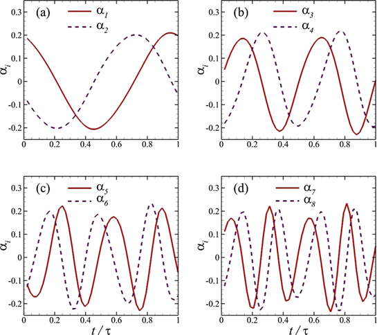
Figure 10. Temporal coefficients for the POD modes of our FSI system at Re = 500.
Download figure:
Standard image High-resolution image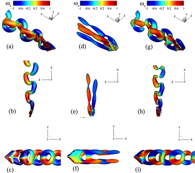
Figure 11. Reconstruction of FSI dynamics for a flow over the caudal fin of a jack fish at Re = 500 using mean features and the POD modes, where the left, middle, and right columns show the full-order fluid–structure dynamics, the addition of the mean states with the POD mode 1, and the addition of the mean states with the POD modes 1 and 2, respectively. Each row shows the perspective, top, and side view of the whole flow and structural domains.
Download figure:
Standard image High-resolution imageNow, we reconstruct the flow and structural dynamics using time-averaged structural states and flow fields and stepwise additions of POD modes to illustrate the contributions of each POD mode towards the production of oscillations in the wake. Using critical values through the Q-criterion here, we provide vortex visualizations where the addition of POD mode 1 with the mean flow and structural fields explains the role of this first oscillatory mode to cause the breaking of the vortex tubes (see figure 6(a)) in the primary direction of the flow. It is evident that the POD mode 1 would play the key role in determining the wavelength of the coherent structures in the wake. Moreover, bringing the POD mode 2 into this system causes the emergence of connecting legs of the vortices to produce coherent flow patterns. For Re = 500, only the mean fields added with the first two POD modes is sufficient to reconstruct the intricate details of the FSI dynamics (see figure 11) although the contribution of these two modes is limited to 70% of the total energy of this system.
Furthermore, we witness that the POD mode 1 computed for Re = 4000 plays the same role in breaking the vortex tubes (not shown here) in the mean flow field (see figure 6(e)). Nevertheless, the addition of another mode (POD mode 2) in this case would not reconstruct the major features of the vortex dynamics as it does for our viscous flow conditions. To develop meaningful connections between the broken parts of the vortex tubes, we need to add at least the first four POD modes into the time-averaged field. The POD modes 2, 3, and 4 play their part for the development and growth of fluidic connections in the lateral and sideways directions to produce significant coherent structures in the wake, as shown by the perspective, top, and side views of the flow domain in figure 12.
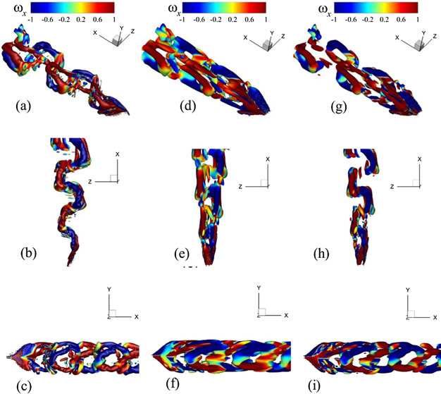
Figure 12. Reconstruction of FSI dynamics for a flow over the caudal fin of a jack fish at Re = 4000 using mean features and the POD modes, where the left, middle, and right columns show the full-order fluid–structure dynamics, the addition of the mean states with the first three POD modes, and the addition of the mean states with the first four POD modes, respectively. Each row shows the perspective, top, and side view of the whole flow and structural domains.
Download figure:
Standard image High-resolution imageHere, column 2 shows the wake constructed from the first 3 modes and exhibits the presence of more intense vortices which is not the case for full-order system dynamics in the 1st column. In the 3rd column, the wake dynamics with the addition of the 4th mode starts resembling more with the full-order system dynamics. It happens due to the phase relationship between the modes that brings the reduced-order representation closer to the full-order one. This dynamical feature can either enhances the strength of vortices or cause a decrease there depending on the constructive and destructive interference between coherent flow structures.
Next, we perform dynamical mode decomposition for the full FSI systems constructed from the structural motion of the caudal fin and the flow field around it. An important objective of this analysis is to segregate the frequency components from each other in this bio-inspired dynamical system where the modes are temporally orthonormal, whereas the temporal coefficient of each POD mode contains more than one frequency. In figure 13, we plot the angular frequencies (rad/ sec) of the DMD modes that are computed by taking the logarithm of Ritz values (DMD eigenvalues) and dividing it by the sampling time interval. Unlike POD, these eigenvalues are not arranged in the descending order, and one needs to carefully determine the significant DMD modes and their associated parameters. A parameter to rank these modes is the amplitude of the DMD modes (Kutz et al 2016). These DMD eigenvalues come up with their complex conjugates because we process the real-valued data here. The Ritz values existing on a unit circle indicate neutrally stable modes, whereas those inside the circle and outside its periphery show decaying and unstable DMD modes, respectively. Here, the real value of an angular frequency (ωr) on the left side of the vertical axis in figure 13 reflects the stability of that particular DMD mode. All the DMD modes with their ωr = 0 are neutrally stable. We neither find any DMD mode with ωr > 0 for Re = 500 nor for 4000. The most dominant mode, in both cases, indicated by red circles in figure 13 are the mean DMD modes also referred to as the DMD mode 1. These modes have ωi = 0 that shows their non-oscillatory character. For Re = 500, the first three strongest oscillatory DMD modes have ωr = 0 which means that they do not decay with time. All the other modes with angular frequencies have negative ωr and decay as we progress in time. This parabolic arrangement of modal frequencies has also been observed previously by Schmid et al (Schmid 2010, 2011). In the case of Re = 4000, only DMD mode 2 has ωr = 0. All the remaining modes show the decaying character. Under both the flow conditions, the DMD mode 2 has the excitation frequency of the caudal fin, whereas DMD modes 3 and 4 have frequencies equal to 2fE and 3fE , respectively.
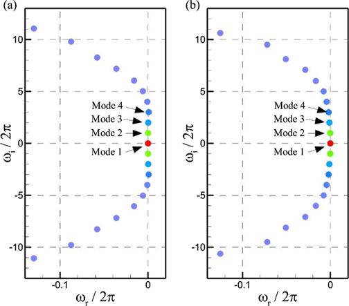
Figure 13. Real and imaginary components of the angular frequencies computed from the Ritz values for (a) Re = 500 and (b) 4000.
Download figure:
Standard image High-resolution imageTo illustrate more on the strength of these DMD modes, we plot frequencies, normalized by the excitation frequency of the caudal fin, and growth rates for each modal component versus modal amplitude in figure 14 for both Reynolds numbers. Here, we only show the information for oscillatory components. We determine that the amplitudes of these frequency components decay asymptotically (see figures 14(a) and (c)), and no DMD mode has a growth rate greater than zero. This element exhibits the stable character of the dynamics of this prescribed fluid–fin interaction-based system. It is important to mention that the strength of higher DMD modes is more in the case of Re = 4000 as compared to those at Re = 500. Modal distributions in figure 14(d) show the cluster of the strongest DMD modes near the zero value on the horizontal axis. Our analysis establishes that the DMD mode 3 contributes more towards the production of thrust force on the caudal fin, whereas the second DMD mode has a greater effect on the lateral force.
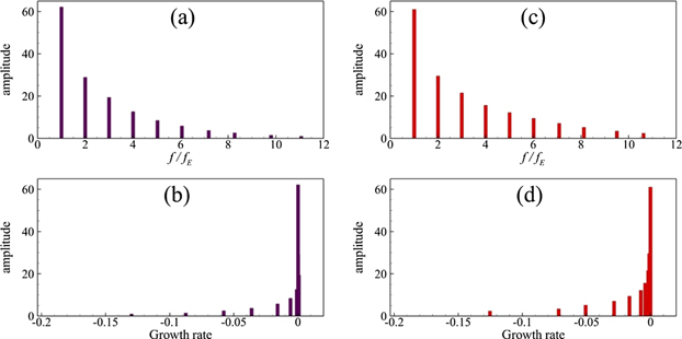
Figure 14. DMD modal frequencies and growth rates vs modal amplitudes for Re = 500 (a) and (b) and Re = 4000 (c) and (d).
Download figure:
Standard image High-resolution imageTo illustrate more on the strength of these DMD modes, we plot frequencies, normalized by the excitation frequency of the caudal fin, and growth rates for each modal component versus modal amplitude in figure 14 for both Reynolds numbers. Here, we only show the information for oscillatory components. We determine that the amplitudes of these frequency components decay asymptotically (see figures 14(a) and (c)), and no DMD mode has a growth rate greater than zero. This element exhibits the stable character of the dynamics of this prescribed fluid–fin interaction-based system. It is important to mention that the strength of higher DMD modes is more in the case of Re = 4000 as compared to those at Re = 500. Modal distributions in figure 14(d) show the cluster of the strongest DMD modes near the zero value on the horizontal axis. Our analysis establishes that the DMD mode 3 contributes more towards the production of thrust force on the caudal fin, whereas the second DMD mode has a greater effect on the lateral force.
As also mentioned by Taira et al (2020), POD and DMD modes are usually similar for periodic flows. In our present study, we observe this phenomenon not only for highly viscous conditions but also at a relatively higher Re ∼ 103. We illustrate these observations by comparing the POD and DMD modes presented in figures 8 and 9 for Re = 500 and 4000, respectively. For the lower Re, the DMD flow structures also appear as planar elements with the four extended arms in the downstream direction, whereas their shapes turn out to be hairpin-like for the higher Re.
To relate our discussion with pressure in the flow fields, we plot the contours of time-averaged pressure coefficient,  , on the caudal fin's surface in figure 15 for both Reynolds numbers. It shows that pressure on both sides exhibits a symmetric pattern under the two flow conditions. However, the distribution of CP is different for these cases. For Re = 500, positive CP region is concentrated on the leading edge of the caudal fin only. We do not find positive CP for Re = 4000 on the tail's surface. Moreover, stronger negative Cp regions are found on the leading edge of the upper lobe and the trailing edge of the lower lobe for the viscous flow regime. In the case of transitional flow condition, the negative CP region expands to the trailing edge of the upper lobe, but it seems concentrated more on the leading edge of the lower lobe. This discussion presents how different Re values can affect the surface pressure distributions on swimmers' bodies and their resultant hydrodynamic forces.
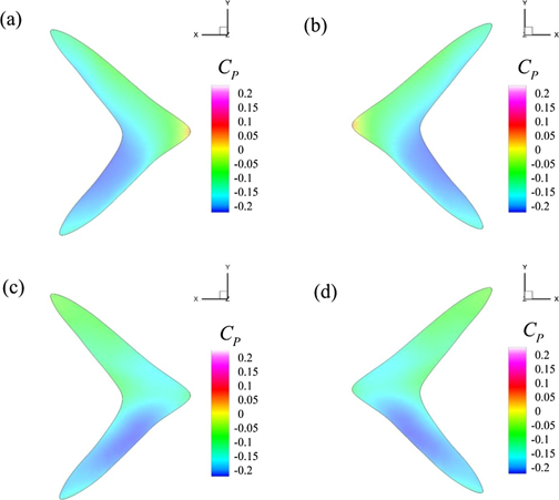
Figure 15. Contours of pressure coefficient on the caudal fin's surface where (a) and (b) show the data for Re = 500 and (c) and (d) presents CP for Re = 4000. Left and right columns are for the right and left sides of the caudal fin, respectively.
Download figure:
Standard image High-resolution imageNext, an effective and interesting method to estimate the hydrodynamic forces is by computing POD modes of the pressure in flow fields around solid bodies. Previously, Imtiaz and Akhtar (2017) proposed this methodology to compute hydrodynamic forces over a cylinder. In this technique, the data matrix is constructed using pressure instead of the velocity components and modal analysis is performed. They did not consider shear stress components to compute hydrodynamic force coefficients and used only the pressure components. Hence, the contribution of each pressure POD mode is determined. Nevertheless, this method has its limitation when drag component due to the friction over the body becomes large. Here, we compare the magnitudes of pressure and drag components, CDP and CDF, respectively, in table 2 for both Reynolds numbers. Their temporal profiles are provided in figure 16 for one oscillation cycle. For Re = 500, CDF makes a greater contribution towards the overall drag production by the caudal fin, and thrust production identified by CDP is not enough to enable the body to generate thrust. In the case of Re = 4000, thrust production from the pressure component overcomes the frictional drag with a small margin. Thus, it demonstrates that we need to form the data matrix by incorporating both pressure and velocity fields information for flows over swimming bodies.
Table 2. Drag force coefficients and their pressure and friction components for Re = 500 and 4000.
| Re | Pressure drag component (CDP) | Frictional drag component (CDF) | Total drag coefficient (CD ) |
|---|---|---|---|
| 500 | −0.1371 | 0.6389 | 0.5018 |
| 4000 | −0.1580 | 0.1358 | −0.0222 |
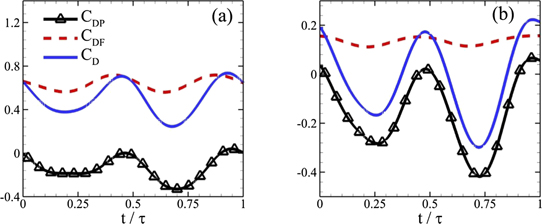
Figure 16. Instantaneous drag coefficient and its components for (a) Re = 500 and (b) 4000.
Download figure:
Standard image High-resolution imageTo further determine the viability of the pressure POD modes in the present flow conditions, we performed the SVD analysis on the following data matrix containing pressure values in a flow field and the caudal fin displacements.
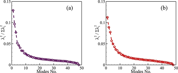
After performing the POD on this data set, we obtain distributions of the normalized energy of the first 48 modes as presented in figure 17 for the two Re values. It is evident that the first mode for lower Re has a greater energy as compared to the one for the higher Re and the higher POD modes start making pairs that are an indication of periodic flows. However, the overall trend of this distribution remains the same. We also observe that the pressure POD technique does not seem suitable for estimating hydrodynamic forces because a very high number of pressure modes, more than 40 in the present work, are needed to capture a significant amount of energy of these dynamical systems. Nevertheless, from this analysis, there arises the need to develop effective and efficient reduced-order models for the direct estimation of forces applied by the fluid on the swimming bodies.
Figure 17. Squared eigenvalues normalized by their summation computed through pressure POD for (a) Re = 500 and (b) 4000.
Download figure:
Standard image High-resolution image
4. Summary and conclusions
In this work, we perform modal decompositions of the kinematics of a jack fish that belongs to the carangiform family of swimmers. We find that its complex undulatory motion is mainly composed of two dominant modes which represent standing waves with different locations of nodes and antinodes along the fish's body and its caudal fin. These two modes are sufficient to present the wavy kinematics of this natural aquatic swimmer and this information can be used to build a low-order model for further studies. Then, we perform numerical simulations for flows over the membranous caudal fin of the jack fish using our immersed boundary method-based computational solver. We employ a large amount of data from this complex FSI system to extract dominant modes using proper orthogonal and DMD techniques. Proper orthogonal decomposition modes provide us with spatially orthonormal structures, whereas the other technique decomposes the entire information about the structural and flow fields into orthonormal frequency components. Each POD mode carries more than one frequency, but each DMD mode has only one frequency. We find that only two modes are sufficient to reconstruct the structural and flow dynamics at the lower Reynolds numbers. However, we need to bring in a greater number of modes to capture essential dynamical features of the flow field at Re = 4000. It means that high modal oscillations occur only due to the fluid dynamics, not the structural motion. We also illustrate the symmetry properties using vorticity components plotted on their respective normal planes in the wakes and reveal that there exists diagonal symmetry for certain POD modes. We also emphasize that these symmetry properties may be switched to asymmetric patterns when their corresponding planes are moved along their normal axes. We find similarities in respective POD and DMD modes for both flow conditions. The coherent structures adopt quadfurcated shapes with four extended arms in the downstream directions in both POD and DMD modes, but we see hairpin-like structures for the flow at the greater Reynolds number. Even these systems are representatives of intense fluid–body interaction, yet we reveal the formation of stable and neutrally stable DMD modes here.
Acknowledgments
M S U Khalid is International Exchange Postdoctoral Research Fellow sponsored by China National Science Postdoc Foundation and Peking University. H Dong acknowledges the support from NSF CNS Grant No. CPS-1931929 and SEAS Research Innovation Awards of the University of Virginia.