

Abstract
The outstanding locomotor and manipulation characteristics of the octopus have recently inspired the development, by our group, of multi-functional robotic swimmers, featuring both manipulation and locomotion capabilities, which could be of significant engineering interest in underwater applications. During its little-studied arm-swimming behavior, as opposed to the better known jetting via the siphon, the animal appears to generate considerable propulsive thrust and rapid acceleration, predominantly employing movements of its arms. In this work, we capture the fundamental characteristics of the corresponding complex pattern of arm motion by a sculling profile, involving a fast power stroke and a slow recovery stroke. We investigate the propulsive capabilities of a multi-arm robotic system under various swimming gaits, namely patterns of arm coordination, which achieve the generation of forward, as well as backward, propulsion and turning. A lumped-element model of the robotic swimmer, which considers arm compliance and the interaction with the aquatic environment, was used to study the characteristics of these gaits, the effect of various kinematic parameters on propulsion, and the generation of complex trajectories. This investigation focuses on relatively high-stiffness arms. Experiments employing a compliant-body robotic prototype swimmer with eight compliant arms, all made of polyurethane, inside a water tank, successfully demonstrated this novel mode of underwater propulsion. Speeds of up to 0.26 body lengths per second (approximately 100 mm s−1), and propulsive forces of up to 3.5 N were achieved, with a non-dimensional cost of transport of 1.42 with all eight arms and of 0.9 with only two active arms. The experiments confirmed the computational results and verified the multi-arm maneuverability and simultaneous object grasping capability of such systems.
Export citation and abstract BibTeX RIS
1. Introduction
Aquatic robots are particularly important for a wide range of underwater applications, such as marine exploration and surveillance, as well as disaster assessment and rescue, suggesting a growing need for higher efficiency, mobility, and agility. The development of sophisticated underwater robotic systems has been inspired, in recent years, by marine organisms that exhibit increased flexibility and adaptability in aquatic environments [1–4]. Aquatic organisms also offer a broad range of locomotion strategies, that are yet relatively unexplored, and could replace conventional thruster technologies, possibly leading to robotic analogues [5–8]. Cephalopod and sea-snake swimming have further encouraged the investigation of alternative propulsion schemes for underwater robots [9–15].
Octopus arms, squid tentacles, elephant trunks, and mammalian tongues are examples of muscular hydrostats [16], which, despite lacking skeletal support, like the bodies of snakes, eels, or arthropods, are still capable of producing a wide variety of dexterous movements and complex shapes as a result of environmental adaptation and ecological diversification. Though not always optimal, each locomotion mechanism has evolved to be efficient within a particular natural habitat. For example, snakes, eels, and worms have developed various modes of terrestrial, arboreal or aquatic locomotion [17], such as sidewinding, concertina and rectilinear. However, lateral undulation (serpentine movement) and peristalsis appear to be the predominant modes for aquatic locomotion in open-sea and in-pipe environments, respectively. Fish swimming has also shown several modes of locomotion depending on speed, shape, and fraction of the body performing undulations (e.g., carangiform, sub-carangiform, and thunniform) [5], of which anguilliform locomotion is the most characteristic of slender fish, like eels. Squid, on the other hand, use both jet propulsion and fin movement to swim, or escape jetting to avoid predators [18]. Octopuses may use their agile arms in various locomotion modes, like crawling or walking on the seabed or for complementing their frequently-employed jet propulsion, in a little-studied swimming mode called arm-swimming or medusoid jetting [19–22]. Although lacking a skeleton, as mentioned, the octopus arms are highly dexterous and can achieve complex shapes and perform several types of movements, such as reaching and fetching, by activating several groups of arm muscles [23–25].
Investigations are currently under way in robotics to develop dexterous manipulators inspired by the morphology and mechanical properties of octopus arms [11, 14, 26–28]. Underwater systems equipped with such manipulators and endowed with multi-function capabilities, would significantly enhance their possible applications. The possibility of using these manipulators for underwater propulsion has not been examined in detail, and is of interest within the context of alternative propulsion mechanisms. The overall goal of the present study is, therefore, to develop a novel bio-inspired underwater robotic platform, which employs a set of such robotic arms primarily for aquatic propulsion, and potentially also for manipulation. The significant redundancy inherent in such a system could enhance the robustness of its operation.
A preliminary study of a planar robotic swimmer, with a pair of rigid arms, assumed an axisymmetric arrangement of the octopus arms during arm-swimming motion, and demonstrated some basic aspects of this mode of swimming [29]. Later studies considered the extension to an eight-arm swimmer [30, 31], equipped with rigid arms, to investigate the propulsive ability of such a system under various forward and turning gaits. A recently developed robotic swimmer considered the effect of a silicone web in between the arms, demonstrating advanced propulsion performance [32]. The main extensions of the present work, with respect to these previous ones, is that here: (i) we investigate propulsion with a set of eight bio-inspired polyurethane-made compliant arms that incorporate a staggered array of octopus-like suckers, (ii) we develop new computational models, which account for this compliance in greater detail, and (iii) we use a single compliant-body robotic prototype swimmer, fabricated via rapid-prototyping methods, as a common experimental validation platform for all forward, backward, and turning gaits considered. Toward this end, we developed lumped-element computational models to study the propulsion generation for a robotic system with eight multi-segment arm-like appendages with flexible joints. A fluid drag model, commonly employed in the robotics literature [33–36], models the interaction of the arm segments with the aquatic environment. Simulations demonstrate the generation of propulsive forces by sculling arm movements. These computational studies are supported by experimental results of a robotic prototype with eight compliant arms inside a water tank. The presented work demonstrates that significant velocity, thrust, and efficiency can be achieved by this bio-inspired robot morphology; its compliance also ensures a smooth and safe interaction with the environment. Moreover, the performance of the compliant robot with respect to its rigid analogues needs not be sacrificed, provided appropriate design and control choices are made, using our computational and experimental studies as guidelines.
Analogous approaches to our multi-arm robotic swimmer are found in the Robojelly and Cyro robots of Virginia Tech [37, 38], and the Festo AquaJelly device [39]. These underwater robots are inspired by the jellyfish, a marine animal that exhibits distinctly different swimming behaviors from the octopus, and achieve primarily straight-line vertical displacements. Compared to these devices, our robotic prototype differs in that it has several controlled degrees of freedom, and is capable of both straight-line and turning movements via a wide range of swimming gaits, which could be exploited toward generating sensor-based reactive behaviors.
The remainder of the paper is organized as follows: section 2 reviews background biological information and finite-element computational models of octopus arm motion. Section 3 presents the more computationally-efficient lumped-element model, developed in Simulink to study parametrically various swimming gaits of the robotic eight-arm swimmer. A series of simulations, which include a parametric study of the effect of the various kinematic parameters on propulsive speed is presented in section 4. Section 5 describes the robotic prototype and presents the experimental studies and the obtained results. Finally, section 6 discusses implications and possible applications of the presented work, as well as some fluid aspects, while section 7 summarizes the results of this study with suggestions for future work.
2. Background studies
Benthic and deep-water octopuses exploit several mechanisms for aquatic propulsion [21]. Arm-swimming or medusoid jetting is a particular swimming mode that octopuses use primarily for defense, hunting, or rapid escape, in addition to jet propulsion. Arm-swimming involves opening and closing of all eight octopus arms and arm crown, in an apparent synchrony, to produce instantaneous bursts of thrust. This behavior has been observed both in the wild, for the Abdopus aculeatus [21], and in the aquarium, for the Octopus vulgaris [22]. The web, mantle, and orientation of the siphon, play an important role during the movement, serving, for example, as steering or buoyancy control mechanisms. The motion of the arms, however, is considered to play the leading role in the generation of propulsive thrust in this mode of swimming.
The kinematics of the octopus arm-swimming motion are complex and exhibit variations, depending on the propulsive speed that the octopus is required to achieve. A fundamental feature [22, 40] is that the motion comprises two strokes, one where the arms, initially trailing behind, open by bending outward relatively slowly (referred, here, as recovery stroke), and one where they return fast to their initial position (referred as power stroke). A series of video frames, illustrating the arm-sculling motion in Octopus vulgaris in an aquarium is provided in figure 1, after background subtraction. We term this two-stroke arm-swimming motion as sculling [30, 31] (see section 4 for the profile description adopted in the robotic model). An estimation of the ratio between recovery stroke and power stroke durations was provided by video recordings of the arm-swimming mode on two Abdopus aculeatus in the wild [21] and five Octopus vulgaris in captivity [22], and was found approximately equal to 2.5 ± 0.5 for both species. There are limited performance data documented in the literature for arm-swimming, jet propulsion or bipedal locomotion for the octopus. Wells et al [41] report, for Octopus vulgaris, jetting speeds of 1000 mm s−1, and walking speeds of 41.6 − 53 mm s−1 ; Huffard calculates average speeds of 453 ± 194 mm s−1 for jetting in the Abdopus aculeatus species [21], and 60 mm s−1 for animals performing bipedal walking with multiple arms (Octopus marginatus) [20]. Video data supplementing [21] indicate a significant burst of activity when the animals employ arm-swimming, however no related speed measurements are provided. Our own studies of arm-swimming motion in the Octopus vulgaris [22, 42] have shown an average speed of 88.42 mm s−1 over a single arm-swimming motion event (without observing any jetting activity) [43].
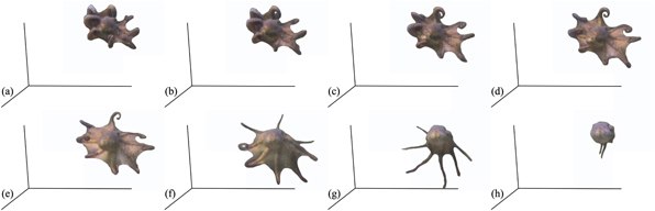
Figure 1. Snapshots from a video recording of octopus arm-swimming motion after background subtraction; (a)–(d) part of the opening phase of the arms, (e)–(h) closing of the arms (power stroke). Axes indicate the corner of the aquarium. Time interval of snapshots: 200 ms [22, 40].
Download figure:
Standard image High-resolution imageOctopus arm muscles consist of fibers and surrounding tissues. These are complex materials and exhibit non-linear, anisotropic, nearly incompressible hyperelastic properties, capable of undergoing large voluntary deformations. Simulation of the mechanical behavior of muscles during activation and deformation is not a trivial task. The first dynamic model of an octopus arm was presented by Yekutieli et al [26]. Based on a three-dimensional, non-linear, implicit finite-element numerical procedure (FEM), we have developed and implemented a detailed computational model for the elastodynamics of the octopus arm, as discussed in detail in [44, 45]. In this model, the stress distribution inside the muscles is considered as the superposition of stresses along the connective tissues and the fibres. The model also takes into account the explicit octopus arm morphology and its continuous nature. This novel approach provides good insight into the generation of complex primitive behaviors, such as fetching, grasping, bending, and reaching, by considering different combinations of muscle groups and activation patterns. However, it is computationally expensive to simulate an entire eight-arm system like the one considered in the present study. In the present paper, therefore, we exploit a lumped-element model (see section 3) to approximate the mechanics of arm movements without taking into account the structure and activation of specific arm muscle groups.
Locomotion within an aquatic environment can be quite challenging, both for biological organisms and for robotic devices. Immersed bodies that are denser than water, like species of cephalopods, may consume considerable energy to produce enough hydrodynamic lift and avoid sinking (buoyancy regulation) [46, 47]. Steady swimming can be achieved by the generation of directional thrust, adequate to prevail upon the induced hydrodynamic drag force and balance the lateral and vertical forces. Estimation of these forces around a swimming octopus and of the thrust-velocity relationship for use in robotic models can be ambiguous since they depend on various factors, e.g., the velocity and the texture. The complexity and deformability of the octopus body shape and arms may also lead to large variations of the induced hydrodynamic loads and to a strong dependance on the corresponding geometrical features. As a result of natural fluctuations in the flow field, the hydrodynamic forces can further be unsteady in time, even in cases in which the body translates at constant speeds (see section 6 for further discussion).
3. Lumped-element dynamical model
Both computational approaches, presented in the previous section, provide valuable insight into the activation mechanisms and thrust generation potential of octopus arms. However, due to the considerable computational load and the lengthy simulation times, they are not very well suited to perform extensive parametric studies or to investigate gait generation strategies for robotic systems. These purposes are better served by lumped-element models, such as the one presented in this section, particularly when the findings of the more detailed computational fluid dynamics (CFD) studies are distilled into them (see section 3.2).
3.1. Mechanical model
The SIMUUN computational environment [36], which is based on the SimMechanics toolbox of Simulink, is used to set up a lumped-element model of an eight-arm system, whose configuration and mechanical parameters are specified to reflect those of the robotic prototype described in section 5. The arms, whose length is denoted by L, are attached to the rear of a mantle-like body shaped as a half ellipsoid with diameter D and half-length D. They are arranged axisymmetrically at 45° intervals, and oriented so that each pair of diametrically opposite arms moves in the same plane (figure 2). Each arm is modeled as a kinematic chain of n = 10 cylindrical rigid segments, interlinked by 1-degree-of-freedom planar revolute joints, whose axis is normal to the arm's motion plane. The joint for the base (i = 1) segment, which connects the arm to the main body in the model, is assumed to be actively driven by an appropriate actuator that enables prescribing a specific angular trajectory for it. Unlike our previous studies [29–31], the segment interlinking joints (i.e., for i = 2..10 in figure 2(b)) are here considered to be unactuated, and feature rotary linear spring-and-damper elements, the parameters of which can be appropriately specified to describe the flexibility of different materials used for the arms (note that active control of the arms' stiffness is not accounted for in this work). For the present study, the arm compliance involved relatively large stiffness for the passive arm joints, which resulted in limited bending motions of the arm, mainly near its tip, during swimming. More specifically, the spring coefficient of the unactuated joints was specified in the range of 0.63 − 0.015 Nm rad−1, gradually decreasing from the arm base toward its tip. Regarding the viscous damping coefficient, a uniform value of  was specified for all of the mechanism's unactuated joints. The preceding values were empirically determined, on the basis of achieving a close match of the simulated arm kinematics with those exhibited by the polyurethane (PU) arms used in the robotic prototype (see section 5).
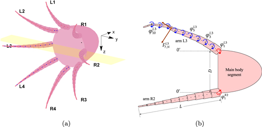
Figure 2. (a) Model of the eight-arm swimmer, indicating the notation adopted for the segmented compliant arms. (b) Planar view of the {L3, R2} pair of diametrically opposite arms, lying on the xy plane. The revolute joints connecting the base arm segments to the main body (shown in red) are actuated, while the other joints are passive, and feature spring-and-damper elements.
Download figure:
Standard image High-resolution image3.2. Fluid drag model
In the developed lumped-element model, the fluid interactions of the mechanical system are described through a simplified resistive fluid drag model. In particular, the modeled system is assumed to move within quiescent fluid so that hydrodynamic forces acting on a single arm segment result only from its motion (i.e., they are not influenced by the motion of neighboring segments). Further, the system is considered to move at speeds at which the generated fluid forces are predominantly inertial ( where the non-dimensional Reynolds number Re characterizes the flow regime). Lastly, it is assumed that the three components of the total flow-induced force (tangential, FT, normal, FN, and lateral, FL) are decoupled. Under these assumptions, the fluid forces describing the interaction of individual arm segments with the surrounding fluid can be expressed as follows:
where vi,T, vi,N, and vi,L are the tangential, normal, and lateral velocity components, respectively, of the ith segment, and λi,T, λi,N, and λi,L are the fluid drag coefficients on the ith segment (i = 1..10), corresponding to each fluid force component. Such resistive fluid drag models originate from studies of swimming animals [48] and are commonly adopted in the robotics literature on bio-inspired elongated underwater systems (e.g., [33–35]). Prior studies by our group, involving detailed CFD analysis of rotating octopus-like arms [29, 49–52], indicate that the underlying assumptions of this fluid drag model are, to a large extent, valid. In addition, the results of these CFD studies have been used to specify the fluid drag coefficients in (1) for the arm segments. The numerical values of λi,dir (listed in mN per m2/s2) are provided in table 1. The distribution of hydrodynamic forces acting along the length of the arm is non-uniform and differs from base to tip [29, 49]. It is also noted that, due to the axial symmetry of the arm segments, the normal and lateral coefficients are equal (i.e., λi,N = λi,L). In addition, the equivalent standard non-dimensional hydrodynamic coefficients Ci,dir are provided in table 2. These were obtained as:

where ρ is the density of water, while Si,dir denotes the projected area of the ith segment for the corresponding velocity component. Since each segment is a cylinder of height hi = L/n and radius ri, the projected areas are calculated as:

Table 1. Numerical values (listed in mN per m2 s−2) of the directional fluid drag coefficients for the 10 segments of each of the mechanism's eight arms.
| i | 1 | 2 | 3 | 4 | 5 | 6 | 7 | 8 | 9 | 10 |
|---|---|---|---|---|---|---|---|---|---|---|
| λi,N | 104.78 | 59.10 | 47.77 | 37.07 | 29.67 | 25.80 | 22.15 | 15.09 | 11.43 | 8.37 |
| λi,L | 104.78 | 59.10 | 47.77 | 37.07 | 29.67 | 25.80 | 22.15 | 15.09 | 11.43 | 8.37 |
| λi,T | 32.63 | 18.41 | 14.88 | 11.55 | 9.24 | 8.03 | 6.90 | 4.70 | 3.56 | 2.61 |
Table 2. Non-dimensional fluid drag coefficients for the 10 segments of each of the mechanism's eight arms.
| i | 1 | 2 | 3 | 4 | 5 | 6 | 7 | 8 | 9 | 10 |
|---|---|---|---|---|---|---|---|---|---|---|
| Ci,N | 0.99 | 0.56 | 0.51 | 0.44 | 0.41 | 0.42 | 0.45 | 0.39 | 0.41 | 0.50 |
| Ci,L | 0.99 | 0.56 | 0.51 | 0.44 | 0.41 | 0.42 | 0.45 | 0.39 | 0.41 | 0.50 |
| Ci,T | 0.19 | 0.11 | 0.11 | 0.11 | 0.11 | 0.14 | 0.18 | 0.21 | 0.31 | 0.62 |
The preceding approach was also used to describe the fluid interactions of the mantle-shaped main body of the mechanism, according to:

where vm,T, vm,N, and vm,L are the tangential, normal, and lateral velocity components, respectively, of the mantle, and λm,T, λm,N, and λm,L are the corresponding fluid drag coefficients. In prior work, the values of these coefficients had been estimated from standard hydrodynamics formulas for flow over an isolated hemisphere [32]. This approach led to considerable quantitative discrepancies between experimental data and the model's predictions, since it does not consider the effect of the arms attached at the rear of the mantle. In the present study, the numerical values of the body drag coefficients were specified on the basis of attaining a good agreement to the simulation results with the experimental data presented in section 5.
4. Gait generation
This section presents a variety of gaits for forward and turning motions of the system, which have been derived from a basic sculling profile for the arms' movements. The key characteristics of these gaits are analyzed by simulation studies with the lumped-element model presented in the previous section.
4.1. Sculling profile
The sculling arm motion involves prescribing a two-stroke periodic angle variation  for the actuated joint connecting each arm to the main body. In the present study,
  is obtained from the following acceleration profile
integrated twice, with  and
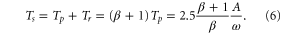
and  , where 2A is the overall angular span and ψ is the angular offset of the sculling motion (figure 3). The preceding formulation results in a smooth motion profile, characterized by sinusoidal acceleration/deceleration phases, which is compatible with the performance characteristics of the actuators employed in the experimental platform, as will be presented in section 5.1. The power (respectively the recovery) stroke velocity is maintained at its maximum value of βω (resp. ω) for 60% of the stroke's duration, while the maximum acceleration for the power (resp. recovery) stroke is β α0 (resp. α0), where
  and a0 = 2πω2/A. The duration of the power and the recovery stroke are obtained as
  and Tr = βTp, respectively. Hence, the overall period of the sculling motion is:
For compliant arms, the angular trajectories of the unactuated joints φi (i = 2..N), and hence the arm's overall shape, evolve in response to the sculling motion of the base segment, the hydrodynamic loads, the joints' flexibility (specified through the parameters of the spring-and-damper elements), and the inertial characteristics of the segments. All of these effects are accounted for by the developed computational tools through the SimMechanics substrate, which derives automatically and solves numerically the dynamic equations of the system.
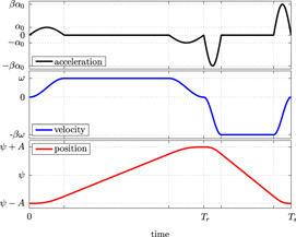
Figure 3. The two-stroke sculling motion profile with a velocity ratio β, where ψ and A denote the angular offset and amplitude of the arms' movement, while ω and a0 correspond to the maximum velocity and acceleration during the recovery stroke, whose duration is denoted as Tr. The period of the overall motion is Ts.
Download figure:
Standard image High-resolution imageThe preceding presented sculling profile can be employed as a basic motion template for the arms to generate a variety of different sculling gaits, for both forward [30] and turning [31] motions of the system, as detailed next.
4.2. Forward gaits
Forward movement along an approximately straight line may be generated by synchronized sculling movements of the robot's arms, employing a variety of patterns of arm coordination. These give rise to patterns of swimming behavior, which, for convenience, will be termed 'gaits'. (This does not imply that transitions among these gaits occur at different velocities, e.g., as in horse gaits.) The timing of the arm coordination patterns, corresponding to each of the gaits described next, are summarized in table 3, which indicates the phase of each arm, as a fraction of the stride period Ts, with respect to arm L1.
Table 3. Definition of sculling swimming gaits with arm coordination patterns
| Arm phase (as fraction of Ts with respect to L1) | ||||||||
| Gait | L1 | L2 | L3 | L4 | R1 | R2 | R3 | R4 |
| G1 | 0 | 0 | 0 | 0 | 0 | 0 | 0 | 0 |
| G2 | 0 | 3/4 | 1/2 | 1/4 | 1/4 | 1/2 | 3/4 | 0 |
| G3 | 0 | 0 | 3/4 | 3/4 | 1/4 | 1/4 | 1/2 | 1/2 |
| G4 | 0 | 1/2 | 0 | 1/2 | 1/2 | 0 | 1/2 | 0 |
G1 gait: The most straightforward arm coordination pattern is when all eight arms perform the sculling motion in synchrony. The arm trajectories are shown in figure 4(a). This gait can be related to the arm-swimming mode observed in live octopuses.
Figure 4. Simulation results: instantaneous axial velocity vb of the main body, shown against the arms' sculling trajectories, for gaits G1, G2, and G4. The dashed red line denotes the average steady-state speed V.
Download figure:
Standard image High-resolution imageG2 gait: This gait is produced by the synchronized sculling movement of pairs of diagonally opposite arms with a phase difference of Ts/4 between adjacent pairs of arms. The trajectories of the four pairs of arms are shown in figure 4(b). Gait G2 results in a smooth forward movement of the robot.
G3 gait: This gait is produced by the synchronized sculling movement of pairs of adjacent arms, in addition to a phase difference of Ts/4 between adjacent pairs of arms. This arm activation pattern gives rise to a relatively slow and wobbling movement of the robot.
G4 gait: This gait is produced by the synchronized sculling movement of two sets of four arms, one set containing arms L1, L3, R2, R4 and the other, arms L2, L4, R1, R3. There is a phase difference of Ts/2 between the two sets of arms. The trajectories of the two sets of arms are shown in figure 4(c).
In the preceding gaits, the action of the arms is equally distributed over the whole duration of the stride period Ts. Numerous variations of the preceding gaits are possible by altering the phase between the arms so that their action is no longer equally distributed over Ts.
The present study focuses on gaits G1, G2, and G4, as these were found to be the most effective for straight-line propulsion. Indicative simulation results, demonstrating forward propulsion by these three gaits, for the compliant-arms system, are shown in figure 4, for ω = 50°/s, β = 5, A = 15° and ψ = 40°. In addition, the snapshots in figure 5 provide an illustration of the arms' bending motion over one sculling period for gait G1. The lower plot of figure 5 shows the orientation angle for the base and the tip of the arm during one sculling period. It can be seen that the orientation of the base segment follows the prescribed angular trajectory  of the active joint, while the orientation of the tip exhibits oscillations superimposed on this profile. These oscillations arise from the flexibility of the arm.
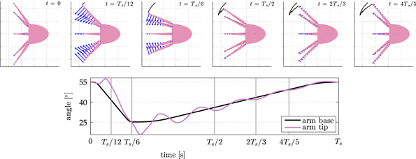
Figure 5. Simulation results: visualization of the compliant-arms system, swimming with gait G1, for A = 15°, ψ = 40°. The blue arrows denote the velocities of the arms' segments, while the black line denotes the trajectory of the tip of arm L3. The snapshots concern different (non-regularly spaced) time instances of one sculling period, whose correspondence with the angular trajectory of the base segment is provided in the lower plot. The latter also shows the orientation of the tip with respect to the main axis of the mechanism.
Download figure:
Standard image High-resolution imageTo aid in the visualization of the proposed sculling-based gaits, a series of animations of the eight-arm mechanism, swimming under gaits G1, G2, and G4, are provided in the accompanying videos of the supplementary material.
The results in figure 4 indicate that, although the average steady-state speed V is approximately the same for the three gaits, the different patterns for the coordination of the arms' sculling motion have a significant impact on the profile of the instantaneous velocity vb(t). In gait G1, vb(t) exhibits quite pronounced peaks that coincide with the occurrence of the power stroke by the arms' synchronized motions. On the other hand, the phasing of the arms' power strokes in G2 results in thrust generation being more evenly distributed over the duration of Ts. The variations of vb(t), which occur with a period equal to Ts/4, are considerably reduced, resulting in a smoother overall forward motion of the system. Correspondingly, the phasing of gait G4 yields a velocity profile with characteristics that fall in between those of the other two gaits. These results are, for the most part, similar to those obtained in our prior study for propulsion with rigid arms [30]. One notable differentiating feature of the response obtained with compliant arms is the high frequency ripples in the instantaneous velocity vb(t) of the system, which are associated with the flexibility of the unactuated joints.
In order to assess the effect of the various kinematic parameters of the sculling profile on the propulsive velocity attained by the compliant-arms swimmer, a series of parametric simulation studies were performed. The parameter space, considered for these simulations, was specified on the basis of the capabilities of the actuators employed in the developed robotic prototype (see section 5.1) to facilitate comparison with experimental results. The results in figure 6(a) show the average steady-state speed V attained by the compliant-arms system in gait G1, when varying the recovery stroke velocity ω and the velocity ratio β, while retaining the sculling amplitude and offset constant ( and ψ = 40°, respectively). As expected, V increases with both β and ω, while forward propulsion is not possible when β = 1. In figure 6(b), the attained speeds from these simulation runs are shown against βω. It can be seen that, at least for the investigated parameter space, the swimming speed is effectively dependent on this quantity, which corresponds to the arms' angular velocity during the power stroke.
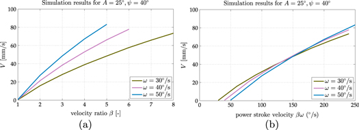
Figure 6. Simulation results: variation of the average attained forward speed V, for gait G1, as a function of (a) the velocity ratio β and (b) the power stroke velocity βω, for different values of ω, when A = 25 ° and ψ = 40°.
Download figure:
Standard image High-resolution imageThe second series of simulations was focused on the effect of the amplitude A and the offset ψ of the sculling motion, retaining constant the other two parameters with ω = 50°/s and β = 5. The results, which are summarized in figure 7, indicate that A has limited influence on the attained speed of the system, particularly for gait G1, while the optimal value for ψ is near 30°. It is noted that the variance of V with respect to ψ, for the compliant arms, is reduced in comparison to what was observed for propulsion with rigid arms in [30].
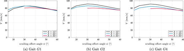
Figure 7. Simulation results: variation of the average attained forward speed V, for the three proposed forward gaits, as a function of the sculling offset ψ, for different values of the sculling amplitude A.
Download figure:
Standard image High-resolution image4.3. Turning gaits
Changes in the overall heading direction of the system can be generated by a variety of asymmetric motions of the robot's arms that result in a range of 'turning gaits'. Multiple such gaits could be implemented by appropriate arm coordination in any three-dimensional direction. It is noted that not all eight arms need to move for the generation of a turning gait; however, non-moving arms were found to facilitate the motion by being held at their maximum angular position.
To systematically study turning on the eight-arm mechanism presented, and facilitate its implementation on the robotic prototype (see section 5), here, we focus our investigation on planar turning gaits using sculling-only movements of the compliant arms. Three such gaits, for turns in the xy plane (with reference to figure 2(a)), are presented next:
GR1 gait: The first turning gait is generated by the synchronized sculling movement of three adjacent arms on the same side of the system, e.g., {L2, L3, L4}, while the remaining five arms are all extended outward, at their maximum angular position, i.e., at (ψ + A). The trajectory obtained with this gait, as well as the temporal variation of the arms' angle and of the turning rate of the main body, is presented in figures 8(a) and (b).
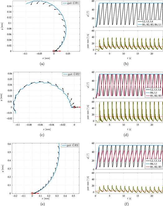
Figure 8. Simulation results for the three proposed turning gaits (obtained with A = 25°, ψ = 30°, ω = 50°/s, β = 5): (a, c, e) trajectory of the center of mass of the main body, over a time span of 16 sculling periods. The initial position of the system at t = 0 is marked with the red circle, and arrows indicate the heading direction of the main body, at the start of each recovery stroke. (b, d, f) Temporal variation of the arms' angle (top), and of the turning rate of the main body (bottom). The dashed red line indicates the average yaw rate at steady state.
Download figure:
Standard image High-resolution imageGR2 gait: In this gait, turning is produced by the synchronized sculling motion of three opposite pairs of lateral arms, namely {R1, L4}, {R2, L3}, and {R3, L2}. The sets of arms {R1, R2, R3} and {L4, L3, L2} rotate sideways in synchrony. The two remaining arms, {L1} and {R4}, are extended outward at the maximum angular position (ψ + A). Simulations illustrating this gait are shown in figures 8(c) and (d).
GR3 gait: The third gait is achieved by the synchronized sculling movement of three opposite pairs of lateral arms, {R1, L4}, {R2, L3}, and {R3, L2}. The three adjacent arms {R1, R2, R3} open and close in synchrony with the opposite set of arms {L4, L3, L2}, while performing the sculling motion at half the amplitude (at the same Ts). Arms {L1} and {R4} are extended outward at the maximum angular position (ψ + A). Indicative results for gait GR3 are shown in figures 8(e) and (f).
The computational framework of section 3 was employed to investigate the characteristics of these turning gaits, through a series of parametric studies. In all of the simulations shown here, the recovery stroke velocity was set at ω = 50°/ s, with a velocity ratio β = 5. Indicative results for the three gaits, obtained with A = 25° and ψ = 30°, are provided in figure 8. The trajectory plots in this figure indicate that gaits GR1 and GR2 essentially implement in-place rotation, with however, different characteristics, particularly with regard to the orientation of the system. On the other hand, gait GR3 appears to be more appropriate for combining heading direction changes with an overall translational motion (see also figure 10). Furthermore, the plots with the temporal evolution of the head segment yaw velocity indicate that the latter exhibits a higher average value, as well as larger variance during each sculling period, for gait GR2.
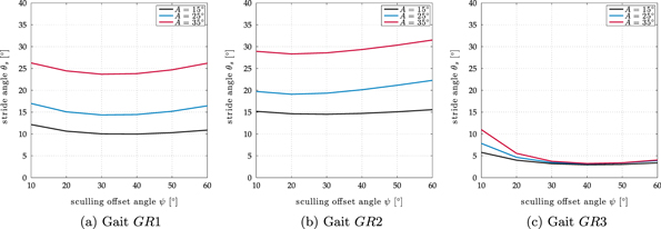
Figure 9. Simulation results: attained stride angle as a function of the sculling offset ψ and the sculling amplitude A, for the three proposed turning gaits.
Download figure:
Standard image High-resolution image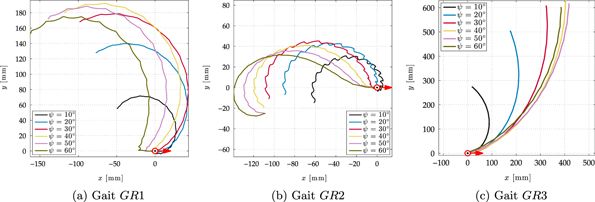
Figure 10. Simulation results: trajectory of the center of mass of the main body, for different sculling offset angles (obtained with A = 25°, ω = 50°/s, β = 5), for the three proposed turning gaits, over a time span of 16 sculling periods (where Ts = 2.1 s). The red circle-and-arrow marker indicates the position and orientation of the system at t = 0. (N.b.: the axis ranges are different in each subfigure).
Download figure:
Standard image High-resolution imageThe stride angle θs, representing the average angle by which the heading direction changes during each sculling period, is provided in figure 9. The results show that, for all three of the investigated turning gaits with compliant arms, θs increases with the sculling amplitude A, while it exhibits little dependence on the sculling offset. It can also be seen that, in line with the observations arising from figure 8, the higher stride angles are obtained with GR2 and GR1, while GR3 is the least effective in incurring rapid changes to the system's heading direction.
In addition, figure 10 shows the effect of the sculling offset angle ψ on the trajectory of the system for the three investigated gaits. The results indicate that, for gait GR1, the overall trajectory of the system is smoother for smaller ψ values, while the opposite is true for gait GR2. Moreover, the turning radius of the trajectory attained with gait GR3 can be seen to be approximately constant for  .
.
As a final comment, we note that the turning performance for all three gaits presented here is influenced considerably also by the hydrodynamic characteristics of the main body, as determined through the drag force coefficients in (4).
5. Robotic experiments
5.1. Experimental setup
For the purposes of this work, a novel compliant-body robotic prototype (figures 11, 12) was developed, based on an octopus-inspired design. The prototype incorporates eight compliant arms, mounted to the rear of a compliant platform, which encloses the battery, electronics, and buoyancy elements (figure 12(a)). All parts are made of PU (PMC-746 urethane rubber) after being cast in purpose-designed molds (figures 12(b)–(d)).
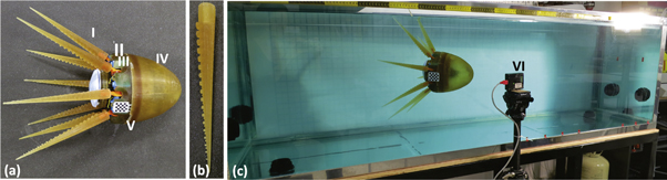
Figure 11. (a) The compliant eight-arm robotic prototype with the PU arms. (b) An individual PU arm. (c) The water tank. Latin numerals are: (I) PU arms, (II) compliant platform, (III) servomotors, (IV) octopus-like mantle, (V) checkerboard marker, (VI) HD camera.
Download figure:
Standard image High-resolution image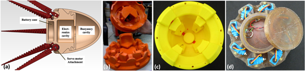
Figure 12. (a) Schematic of the robotic prototype indicating the internal cavities. Custom-designed molds for: (b) the platform and (c) the mantle. (d) The cast PU platform with the servomotors in place and the battery space.
Download figure:
Standard image High-resolution imageThe arms are conical, with length of 200 mm, base radius of 10 mm, and tip radius of 1 mm, and include 38 cylindrical sucker-like protrusions along their length. The latter are arranged in a staggered configuration, covering about one-third of the arm's surface area [49, 51]. Each arm is driven by a dedicated waterproof micro-servomotor (HS-5086WP, Hitech, USA) that allows a 110° span of rotation. The arms are arranged symmetrically at the rear side of the platform (inserted in custom-made compartments, figure 12(d)), such that diametrically opposite arms move in the same plane and with the protrusions side facing inward. The platform is circular with a diameter of 16 cm, while the octopus-like mantle is a half ellipsoid with major and minor axes of 16 cm and 8 cm, respectively. The mantle encloses an empty cavity that can be filled with water to adjust the buoyancy of the robot (figure 12(a)). The overall weight of the submerged prototype with the buoyancy cavity filled with water is 2.68 kg. The compliant parts of the robot were cast in molds (figures 12(b) and (c)) that were custom designed in SolidWorks® and fabricated in ABSplus material, using a three-dimensional printer (Dimension Elite, Statasys, USA). A mixture of liquid urethane was poured in the molds, at room temperature, avoiding air entrapment, and was left overnight to cure. The material's specific gravity is 1.035 g/cc, while its dynamic viscosity is 5 kg m−1s−1; the tensile strength is 4.826 N mm−2, with a Young's modulus E of 3.605 N mm−2. Evidence from analytical models of stiffness in uniform cylindrical beams shows that the stiffness increases fast, in a non-linear manner, as a function of the radius of the beam. This is consistent with the variation of the stiffness from base to tip of the arm that we employed in the simulation studies.
The robotic prototype is energetically autonomous, being powered by an on-board Li-Po battery that allows for about 1 hour of continuous operation. It is also fully untethered and tested underwater in an experimental water tank of length 200 cm, width 70 cm, and height 60 cm. An 8-bit microcontroller platform (Arduino pro mega) is used to program the arm trajectories for implementation of the various swimming gaits, and to collect data regarding the electrical power consumption of the servos. Communication between the microcontroller and a local PC is achieved wirelessly through a dedicated RF link (RFM22B-S2), operating at 433 MHz ISM.
The position and orientation of the robotic prototype inside the water tank are estimated by computer vision methods with a high-definition camera (at 25 fps). A checkerboard marker of known size (figure 11(a)) is placed on the robot during the experiments. The pose of the marker is estimated in each camera frame by calculating the homography between the camera's image plane and the marker's plane, up to a scale factor.
In addition, a custom test-rig, shown in figure 13, has been set up to measure the forces generated by the arm-swimming gaits. A high-precision digital force gauge (Alluris FMI-210A5) is mounted on top of a dexion frame and placed in the water tank such that the dynamometer lies above the water's surface. The generated force from the submerged robot is transmitted to the dynamometer via a rigid stainless steel shaft, acting as a lever. The lower end of the lever is attached to the platform, while the upper end pushes against the force gauge. A spherical bearing is placed at the lever's fulcrum, positioned at the point where the ratio of power transmission is half. All orange parts shown in figure 13 have been fabricated in ABSplus material. This setup allows measurement of forces generated by the arm motions while the robot is restrained from moving. The measurement data are acquired from the force gauge via a custom interface running under LabView in the host PC.

Figure 13. The experimental setup employed for measuring the axial force generated by the mechanism.
Download figure:
Standard image High-resolution image5.2. Forward propulsion results
Here, we present experimental results from a series of tests to assess the propulsion performance of the robotic prototype, equipped with the compliant PU arms, under the various arm-swimming sculling gaits G1, G2, and G4 presented in section 3. The conducted tests confirmed the generation of forward propulsion for all three of the investigated gaits. Figure 14 displays snapshots from one test run, with the prototype swimming using gait G1. Indicative results for the displacement and the velocity profile of the robot swimming in gaits G1, G2, and G4, using the same sculling parameters, are shown in figure 15. As indicated in these graphs, the qualitative characteristics of the velocity profiles, associated with each gait, were found to be consistent with those identified in the simulation studies (see section 4.2). We also note that a 'twitching' of the compliant arms during their recovery stroke, which was particularly evident for G1, was visually observed during these tests. This is consistent with the high frequency ripple in the instantaneous velocity profiles in the simulation results (see figure 4). The fact that a similar ripple does not appear so prominently in the experimental data shown in figure 15 is attributed to the vision-based method employed to track the motion of the prototype.
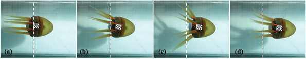
Figure 14. Forward propulsion of the robotic prototype for gait G1 (A = 25°, ψ = 25°, ω = 50°/s and β = 5). Frames are shown with a constant time interval of 542 ms (accompanying video in supplementary material).
Download figure:
Standard image High-resolution image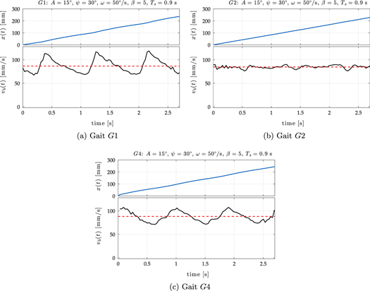
Figure 15. Experimental results of forward propulsion with compliant PU arms, for swimming in the three investigated gaits, with A = 15°, ψ = 30°, ω = 50°/s, and β = 5. Each panel shows the robot's displacement (upper plot) and the corresponding velocity profile (lower plot), over a time span of three sculling periods (where Ts = 0.9 s) at steady state. The dashed red line in the lower plot indicates the average steady-state velocity.
Download figure:
Standard image High-resolution imageThe data shown in figure 16 summarize the average speed V attained by the robot in gaits G1, G2, and G4, for different A and ψ values, when ω = 50°/s, and β = 5. For comparison purposes, the experimental data (denoted by solid lines with circular markers) are shown along with the simulation results (denoted by dashed lines), already presented in figure 7. The experimentally obtained values for V are, for all three gaits, in the range of approximately 70−100 mm s−1, exhibiting moderate dependence on the sculling amplitude A, particularly for gaits G2 and G4. It can be seen that the simulation studies are quite effective in predicting the velocity of the system for gait G2, while more significant discrepancies appear for G4 and, even more so, for G1. It is noted that the latter two gaits are associated with a more discontinuous motion of the system (see figure 15). This suggests that the observed discrepancies are due to inherent limitations of the simple drag model employed for the fluid interactions of the system, which manifest themselves to a larger extent during unsteady phenomena.
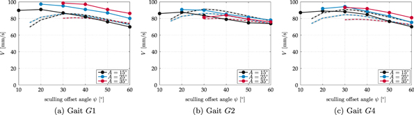
Figure 16. Forward propulsion results: average speed attained by the robot with the use of the compliant arms, for the three investigated gaits (ω = 50°/s, β = 5). The experimental data (solid lines with circular markers) are shown along with corresponding simulation results (dashed lines).
Download figure:
Standard image High-resolution imageIt is also of interest to note that, unlike the simulations, the experimental results indicate a slight shift of the optimal ψ value with A. Motivated by this observation, figure 17 plots the speed of the system against ψ − A (rather than ψ). The combined variable ψ − A provides a clearer picture of the system's behavior. It can be seen to effectively render the speed independent of the sculling amplitude, with the velocity being maximized when ψ − A is near zero. This suggests that, to optimize the forward speed for given β and ω values, the sculling offset should, in practice, be specified to be equal to the sculling amplitude.

Figure 17. Experimental results: the average forward speed of the system (see figure 16), shown against ψ − A (ω = 50°/s, β = 5).
Download figure:
Standard image High-resolution imageAn additional set of measurements was performed, with the robot swimming in gait G1, whereby the sculling amplitude and offset were held constant ( and ψ = 30°), while varying the velocity ratio β and the recovery stroke velocity ω. The forward speeds attained by the robot during these tests, for three different ω values, are summarized, along with corresponding simulation results, in figure 18. It can be seen that the model underestimates the robot's velocity by about 10%, a discrepancy that, as explained previously, could be attributed to the unsteady characteristics of the system's motion in gait G1. Nevertheless, it should be pointed out that the experimental results confirm the simulations' prediction that the main control variable, upon which the forward swimming velocity depends, is the arms' power stroke angular velocity βω (see figure 18(b)).
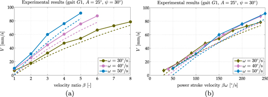
Figure 18. (a) Variation of the average attained forward speed V, for gait G1, as a function of the velocity ratio β, for different values of the recovery stroke velocity ω, when A = 25° and ψ = 30°. The experimental data (solid lines with markers) are shown along with corresponding simulation results (dashed lines). (b) The same data, shown against βω (i.e., the arms' angular velocity during the power stroke).
Download figure:
Standard image High-resolution image5.2.1. Cost of Transport (CoT)
The propulsive efficiency of the developed prototype is examined here using the non-dimensional cost of transport (CoT) metric, calculated as

where Pin denotes the average electrical power consumed by the servos driving the arms during a sculling period, m is the mass of the swimming platform with the eight compliant arms, g is the acceleration of gravity, while V is the average steady-state swimming velocity.
A summary of the thus estimated CoT values, derived from the parametric studies for the three gaits (see figure 16) is provided in figure 19. It can be seen that, for all three gaits, the CoT generally lies in the range between 1.5 and 2.0, exhibiting limited variance with respect to the sculling amplitude A. Moreover, figure 20 shows the variance of the CoT with respect to β and ω, derived from the measurement set in figure 18, involving different β and ω values. The results indicate that the efficiency of propulsion increases considerably with the velocity ratio β.

Figure 19. Experimental results for forward propulsion: average CoT for the three investigated gaits, shown as a function of ψ and A (ω = 50°/s, β = 5).
Download figure:
Standard image High-resolution image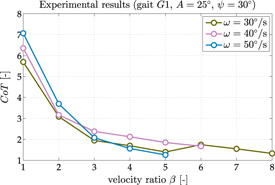
Figure 20. Experimental results: estimated CoT for propulsion in gait G1, as a function of the velocity ratio β, for different values of the recovery stroke velocity ω when A = 25° and ψ = 30°.
Download figure:
Standard image High-resolution image5.2.2. Effect of number of active arms
An additional set of measurements was performed with the eight-arm swimmer to investigate the propulsion characteristics of the system with respect to the number of arms participating in propulsion. The conducted tests involved swimming in gait G1 with varying ψ values, while employing only two or four arms, with A = 25°, ω = 50°/s, and β = 5. The inactive arms were held at an angle of 0° (this requires some energy consumption).
The results of these measurements, compared against those obtained for swimming with all eight arms, in terms of the attained speed V, the overall power consumption Pin, and the CoT, are provided in figure 21. In can be seen that, for fewer arms participating in propulsion, the CoT becomes essentially independent of the sculling offset angle. The mean CoT, averaged over the range of ψ values, is approximately 0.98 for two arms, 1.07 for four arms, and 1.63 for eight arms.
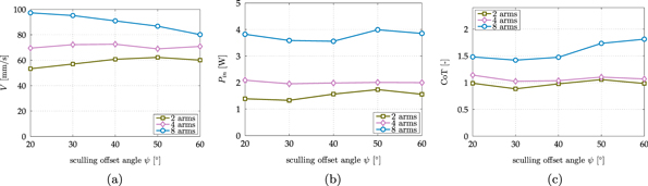
Figure 21. Experimental comparison of the performance of two, four and eight arms in the eight-arm swimmer: (a) propulsion speed, (b) power consumption, and (c) estimated CoT, for swimming in gait G1, as a function of the sculling offset ψ (A = 25°, ω = 50°/s, and β = 5).
Download figure:
Standard image High-resolution imageThe observed rise in the cost of transport as the number of arms increases is consistent with other results for the CoT in multi-appendage aquatic robots [53]. It can be attributed to the fact that, as the number of arms is increased, the average swimming velocity also increases. In turn, this entails a larger hydrodynamic resistance during the arms' recovery stroke, which places higher demands in the servomotors driving the arms. Since this resistance scales quadratically with velocity, the increase in the power requirement Pin, is more substantial than the increase in velocity attained by employing more arms for propulsion (see figures 21(a) and (b)).
It is noted that, since figures 16 and 19 indicate that the average attained velocity and the cost of transport are approximately the same for eight-arm swimming in the three investigated forward gaits (assuming a given set of the arms' sculling motion parameters), we expect that the preceding findings regarding the variance of the CoT with respect to the number of arms also apply to gaits G2 and G4.
5.2.3. Propulsive forces
Indicative plots for the axial force measurements obtained with the eight-arm system are shown in figure 22. It can be seen that, although the average generated force is approximately the same for all three gaits, the instantaneous force profiles exhibit marked differences. Similar to the free-swimming velocity profiles (see figures 4 and 15), these can be attributed to the different phasing of the arms' power stroke in the three gaits. More specifically, the generated force under gait G1, where all eight arms move in synchrony, exhibits a single large positive peak during each sculling period. In G2 there are two distinct such peaks, of a lesser amplitude in comparison to G1, related to the fact that the arms move in two sets of four. Finally, the phasing of the arms' power strokes in G2 results in thrust generation being evenly distributed over the duration of the sculling period. In addition, figure 23, shows the average magnitude of the positive force peaks, recorded for G1, as a function of ψ + A (i.e., the angle of the arms when the power stroke is initiated). As would be expected, higher peak forces are attained along the axial direction with increasing ψ + A values.
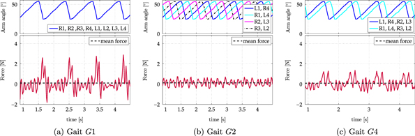
Figure 22. Axial force measurements for forward swimming in gaits G1, G2, G4 (A = 15°, ψ = 40°, ω = 50°/s, β = 5). The dashed line denotes the average force.
Download figure:
Standard image High-resolution image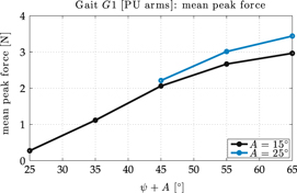
Figure 23. Mean peak force for forward arm-swimming using the compliant PU arms, for gait G1, as a function of the power stroke initial angle ψ + A, for different values of the sculling amplitude A (ω = 50°/s, β = 5).
Download figure:
Standard image High-resolution image5.3. Turning motion results
Experimental results obtained with the eight-arm robotic prototype are presented for the turning gaits GR1, GR2, and GR3, prescribed as in the computational studies. Figure 24 displays snapshots from an indicative case for gait GR1 (A = 25°, ψ = 25°, ω = 50°/s and β = 5). Initially, the robot is parallel to the long side of the tank and then it performs a clockwise turn of approximately 70°, achieved over six sculling periods (corresponding to 10.5 s).
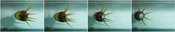
Figure 24. The eight-arm robotic swimmer performing the turning gait GR1 (A = 25°, ψ = 25°, ω = 50°/s, β = 5, and Ts= 1.75 s), at snapshot intervals of two sculling periods: t = (a) 0, (b) 2Ts, (c) 4Ts, (d) 6Ts (accompanying video in supplementary material).
Download figure:
Standard image High-resolution imageEstimates for the average stride angle of the robotic swimmer, obtained from the analysis of the vision system data, are provided for the three gaits in figure 25, as a function of the sculling amplitude and sculling offset. Along with the experimental data (denoted by solid lines with markers), the plots also show the results from corresponding simulation runs (denoted by dashed lines). Although there are quantitative differences, the experimental data indicate that the model captures effectively a number of characteristics related to each of the studied gaits. In particular, it can be seen that the stride angles for gaits GR1 and GR2 are similar and larger than the ones for gait GR3. Moreover, the experimental data also confirm the predictions of the simulations, regarding the reduced dependency of the stride angle on the sculling amplitude for GR3, compared to the other two gaits.

Figure 25. Attained stride angle of the robot as a function of the sculling offset ψ and the sculling amplitude A, for the three proposed turning gaits (ω = 50°/s, β = 5). The experimental data (solid lines with circular markers) are shown against corresponding simulation results (dashed lines).
Download figure:
Standard image High-resolution imageIt should be noted that certain shortcomings of our experimental setup (e.g., boundary effects due to the limited width of the water tank, and difficulties in the acquisition of the visual data due to the limited field of view of the underwater camera) have a more significant impact when studying turning maneuvers, compared to forward swimming, and may have contributed to the discrepancies between the experimental data and the simulation results observed in figure 25.
6. Discussion
The present study addresses an alternative propulsion mechanism for underwater locomotion, inspired by the octopus. It concentrates on the relatively unknown arm-swimming motion of the octopus as a unique mode of locomotion, in which the animal also uses its manipulator arms for propulsion. We approximate this motion via both computational modeling and the development of a robotic prototype, fabricated primarily from compliant materials and used to investigate a range of gaits for forward propulsion and turning. The underwater experiments performed demonstrate the efficiency of the swimmer, in terms of the attained velocities (maximum average velocity: 98.6 mm s−1, or equivalently 0.26 body length per second, for a body length of 380 mm for the entire system), the generated propulsive forces (maximum instantaneous axial force: 3.5 N) and the CoT (optimal CoT with eight arms: 1.42; with only two active arms: 0.9). The performance of our prototype is comparable to other multi-limb underwater robots, e.g., the Cyro robot with a non-dimensional CoT of 1.11 and average velocity of 84.7 mm s−1 [38], and the Madeleine four-flippered robot with a CoT approximately equal to 0.5 [53]. It is also comparable to the speeds (approximately 90 mm s−1) observed for the Octopus vulgaris performing arm swimming in our studies with live animals [43], as described in section 2).
In addition, we investigated the generation of various gaits for both forward propulsion and turning. Gait investigation is an important issue in animal and multi-limb robot locomotion studies [53]. The Octopus vulgaris uses various modes of locomotion depending on its intended behavior [21]. However, it is not yet clear what event might trigger the arm-swimming behavior. The primary context for both appears to be hunting or escape. Our investigation on the different swimming gaits originates from a general robotic interest in multi-limb underwater locomotion. For example, it is not so obvious how different combinations of arms produce a specific range of forces and motion trajectories. If different gaits can generate similar attained velocities, then it remains as an open question why the octopus is not known to exhibit an even greater variation of swimming modes.
Further to forward propulsion and turning gaits, as demonstrated in section 5, our eight-arm robot exhibits several additional capabilities. These could serve toward current and emerging realistic robotic underwater applications, and could point to a versatile aspect of multi-functional, multi-arm underwater robotic devices, as discussed briefly in the following paragraphs (accompanying videos are provided as supplementary material).
6.1. Combination of maneuvers
By sequentially activating forward and turning gaits, it is possible for the system to move along complex paths. One such example is provided in figure 26, in which the robot describes a right-angle path by initially employing gait G1 to move forward, then switching to gait GR2 to perform a turning maneuver, and finally reverting to G1 for the last part of the motion. Similar combinations of the forward and turning gaits presented in the previous sections can be employed by the robotic swimmer, providing a range of combined trajectories. The ability to combine various straight-line and turning maneuvers, provides the system with the capacity to navigate along complex paths. This highlights the potential of implementing reactive behaviors, e.g., collision avoidance, pipe following, etc, that are important for underwater applications.

Figure 26. Robot trajectory obtained by sequencing movements in forward and turning gaits, over a total of 50 sculling periods with A = 25°, ψ = 35°, ω = 50°/s, and β = 5. The black line indicates the trajectory of the main body segment.
Download figure:
Standard image High-resolution image6.2. Backward propulsion
Backward propulsion can also be obtained by modifying the timing of the sculling motion so that the power stroke occurs when the arms are extended toward the mantle, while the recovery stroke is performed during closing of the arms. This motion can be employed both in simulation and experimentally, as shown in the snapshots of figure 27. Here, the swimmer swims backward (i.e., arms first), by reversing the power and recovery strokes in the sculling profile. The ability of a robotic agent to perform both forward and backward propulsion, with similar efficiency, may have particular importance to inspection, and search and rescue applications.
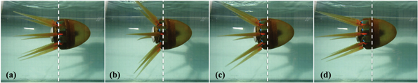
Figure 27. Backward motion of the robotic prototype by using all eight arms with a reverse G1 sculling gait (A = 15°, ψ = 35°, ω = 50°/s, and β = 5). Frames are shown with a constant time interval of 334 ms (accompanying video in supplementary material).
Download figure:
Standard image High-resolution image6.3. Grasping
To highlight the potential of employing the arms both for propulsion and for manipulation, figure 28 provides a series of snapshots from an experiment in which two of the robot's arms (specifically, the diametrically opposite pair of arms L1 and R4) are employed in grasping an object (here, a plastic ball), while the other six are allocated to the propulsion of the system, implementing the G1 forward swimming gait. Depending on the overall dimensions and weight of the object, additional arms could be allocated to grasping. The compliance of the arms is of key significance for such schemes, as it allows for a safe and shape-adaptable handling of objects.

Figure 28. Manipulation capabilities of the robotic prototype by using a pair of arms to grasp an object. The remaining six arms implement the G1 forward swimming gait (A = 15°, ψ = 40°, ω = 50°/s, and β = 5). Frames are shown with a constant time interval of approximately 292 ms (accompanying video in supplementary material).
Download figure:
Standard image High-resolution image6.4. Other aspects of experimental and computational studies
It can be seen that our experimental results largely support the predictions of the lumped-element models proposed, which, although simplified, appear to be in good agreement with the robotic experiments, capturing adequately the behavior of the system in the operating envelope considered. Various discrepancies, between the experimental results and the simulation ones, may be due to inaccuracies in the specification of the modeling parameters, limitations of the fluid drag model used, imperfect buoyancy compensation, inherent limitations and performance variability of the servomotors used in the prototype, as well as limitations in the computer vision estimation methods used.
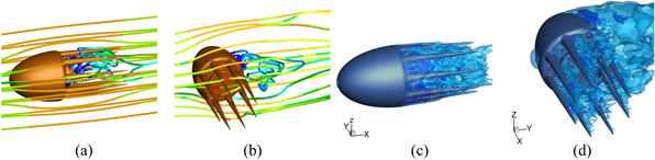
Toward expanding our array of computational tools for the analysis of the system, we are currently considering employing CFD methodologies for the numerical study of the time-dependent flow around the full robotic system, comprising the mantle and eight sculling arms, under the various proposed gaits. Such an approach would provide better insights regarding the coupling between the system and the surrounding fluid, the effect of which is not captured by the simple fluid drag models used in the lumped-element simulation tools. To this end, we present here indicative results from two preliminary CFD analyses, involving two different simplifications of the system [49, 51, 52]. The first one considers a single-arm self-propulsion system performing a two-stroke sculling motion (figures 29 and 30), that demonstrates the generation of forward thrust. The unsteady flow solution was obtained utilizing high-accuracy numerical methodologies (details in [51]). The sculling arm follows the motion profile described in section 4.1, while rotating as a straight unit around its base and sliding freely along the x-axis. A comprehensive analysis of the observed vortical structures is provided in [51]. The generated hydrodynamic force along the x-axis is shown for this case in figure 30(a), along with the attained velocity  and displacement
  over the duration of 5 cycles (figure 30(b)). These results exhibit similar trends to those demonstrated by the computational and experimental results of sections 4 and 5, respectively.

Figure 29. CFD studies: Top row: isocontours of instantaneous vortical structures generated around a self-propelling octopus-like sculling arm, able to slide along the x-axis for A = 20°, ψ = 40°, ω = 50°/s, and β = 5 [51]. Bottom row: corresponding instantaneous arm locations with respect to the starting position for the current cycle (marked with circle and triangle). (a) 0.26 Ts, (b) 0.52 Ts, (c) 0.78 Ts, (d) 0.9 Ts, (e) Ts = 1.04 s.
Download figure:
Standard image High-resolution image
Figure 30. CFD studies: (a) Hydrodynamic force in the direction of propulsion for a self-propelling octopus-like sculling arm. (b) Propulsive speed  and displacement
  over the duration of five cycles. The sculling parameters are listed in the legend of figure 29 [51].
Download figure:
Standard image High-resolution imageIn addition to the above, we considered a CFD study of the entire system of the mantle and non-moving arms, translating at a steady speed within quiescent fluid (figure 31). The figures reveal a complex flow disturbance in the surrounding region for both forward and lateral motion (equivalently, for both flow directed toward the mantle tip and the lateral side) and demonstrate the effect of the mantle on the motion.
Figure 31. CFD studies: (a, b) velocity streamlines and (c, d) isocontours colored by velocity magnitude around a stationary octopus-like mantle, for a free stream velocity of 0.1 m s−1 (dark blue denotes low values, and red high). The flow is directed from left to right, either (a, c) toward the mantle tip, or (b, d) toward its lateral surface.
Download figure:
Standard image High-resolution image
7. Conclusions
The present study investigates robotic swimming by multiple compliant arms, inspired by the octopus, via both computational modeling and the development of a robotic prototype fabricated primarily from compliant materials. The underwater experiments performed demonstrate the flexibility and efficiency of the swimmer. Our interest was to examine the possibility of obtaining robotic swimming based solely on the movements of the arms. This falls within a general robotic interest of investigating alternative mechanisms of aquatic locomotion. Our experimental studies also demonstrate the possibility of using the arms for manipulation as well as for propulsion. This ability could be significant in the context of demanding underwater robotic applications, such as inspection of underwater structures, search and rescue operations, and marine ecosystem monitoring. Furthermore, work is currently underway to develop appropriate neural networks for the generation of rhythmic behavior, capable of producing the basic sculling profile and the relative phasing associated with each of the proposed gaits, via simple modulation commands. Future work will also address the refinement of our models, including more detailed CFD studies, the investigation of the stiffness relationship for our compliant arms, the addition of more controlled degrees of freedom in each compliant arm for better replicating the arm kinematics extracted from animal recordings, and the implementation of active buoyancy control. Sea swimming tests and studies of robot–fish interaction in real marine ecosystems will also be investigated.
Acknowledgments
This work was supported in part by the European Commission (EC) via the ICT-FET OCTOPUS Integrated Project (No. 231608), by the EC/ERDF and the General Secretariat for Research and Technology (GSRT) of the Hellenic Ministry of Education via the BIOSYS-KRIPIS project [MIS-448301 (2013SE01380036)], by the ESF-GSRT HYDRO-ROB Project [PE7(281)], as well as by Greek national funds through the Operational Program Education and Lifelong Learning of the National Strategic Reference Framework (NSRF)—Research Funding Program: THALES via the BioLegRob Project (Mis: 379424). Parts of the CFD simulations were carried out on the CaSToRC High-Performance Computing (HPC) system of the LINKSCEEM/Cy-Tera resources (Project pro14a108) and the PRACE Tier-1 HPC system (Project CepFlow, 12DECI0048). The authors would like to thank B Hochner, M Kuba, T Flash, F Grasso, P S Krishnaprasad, and J A Ekaterinaris for insightful discussions. We are also grateful to A Chatzidaki, T Evdaimon, and V Koussanakis for their assistance with these studies, as well as X Zabulis, P Pandeleris, and S Stefanou for their assistance with computer vision issues.
Accompanying videos of simulation and experimental results appear in supplementary material.