

Abstract
The genetic code is redundant, as there are about three times more codons than amino acids. Because of this redundancy, a given amino acid can be specified by different codons, which are therefore considered synonymous. Despite being synonymous, however, such codons are used with different frequencies, a phenomenon known as codon bias. The origin and roles of the codon bias have not yet been fully clarified, although it is clear that it can affect the efficiency, accuracy and regulation of the translation process. In order to provide a tool to address these issues, we introduce here the codon information index (CII), which represents a measure of the amount of information stored in mRNA sequences through the codon bias. The calculation of the CII requires solely the knowledge of the mRNA sequences, without any other additional information. We found that the CII is highly correlated with the tRNA adaptation index (tAI), even if the latter requires the knowledge of the tRNA pool of an organism. We anticipate that the CII will represent a useful tool to study quantitatively the relationship between the information provided by the codon bias and various aspects of the translation process, thus identifying those aspects that are most influenced by it.
Export citation and abstract BibTeX RIS
1. Introduction
Molecular biology is undergoing profound changes as major advances in experimental techniques are offering unprecedented amounts of data about the molecular components of living systems [1]–[4]. Most notably, the analysis of the thousands of genomes that have been sequenced [4] is revealing the mechanisms and principles through which the genetic information is maintained and utilized in living organisms [5]–[8].
A question of central importance concerns the causes and consequences of the redundancy of the genetic code. During translation, each amino acid is specified by a triplet of nucleotides (a codon). A given amino acid, however, may correspond to more than one codon, so that 61 codons correspond to 20 amino acids. For instance, lysine is encoded by two codons, valine by four and arginine by six. The way in which these synonymous codons are used shows a marked bias, a phenomenon known as codon bias [9, 10]. For instance, in humans, for the amino acid alanine the codon GCC (guanine–cytosine–cytosine) is used four times more frequently than the codon GCG. The codon bias is characteristic of a given organism and has been associated with three major aspects of mRNA translation, which are efficiency, accuracy and regulation [10, 11].
The first aspect is efficiency. The codon bias and the tRNA abundance in a given organism appear to have co-evolved for optimum efficiency [12]–[14]. Since synonymous codons can be recognized by different tRNAs and translated with different efficiencies, the codon bias is related to the translation rates [15]–[18]. Moreover, codon usage has been shown to correlate with expression levels [19]–[26], so that the use of particular codons can increase the expression of a gene by up to two or three orders of magnitude [27, 22].
The second aspect is accuracy. The codon bias can be used to control the accuracy in the translation, an effect that appears to have been optimized to reduce misfolding and aggregation [28].
The third aspect is regulation. Different codon choices can produce mRNA transcripts with different secondary structure and stability thus affecting mRNA regulation and translation initiation [22, 29]. The codon usage has also been associated with the folding behaviour of the nascent proteins, by timing the co-translational folding process [30].
Since all these aspects of the translation process rely in some form on the information provided by the codon bias, in this work we address the question of establishing a measure of the amount of information encoded in the codon bias itself. For this purpose, by using a combination of statistical mechanics and information theoretical techniques, we introduce the codon information index (CII).
An immediate question is about the need of a new measure associated with the codon bias, when several measures for it have already been proposed, including the 'effective number of codons' ( ) [31], the 'frequency of optimal codons' (Fop) [12], the 'codon bias index' (CBI) [20], the 'codon adaptation index' (CAI) [32], and the 'tRNA adaptation index' (tAI) [33]. Among these measures, the CII is specifically designed to describe the amount of information encoded in mRNA sequences through the codon bias, and it is the only one with the following properties: (i) it requires only information about the mRNA sequences and does not depend on any additional data, i.e. the CII is self-contained, and (ii) it produces a codon-wise profile for each sequence which is sensitive to the spatial organization of the codon. As examples, we mention in particular that, for a given organism, the tAI requires the knowledge of the tRNA pool, and that the CAI requires the knowledge of the most expressed genes.
We first analyse the general properties of the CII and then we apply it to a pool of 3371 genes of yeast. We find that the CII correlates with protein and mRNA abundances, as well as with the tRNA adaptation index (tAI) [33]. The latter result shows that two independent forms of information, which are stored in different parts of the genome, the tRNA copy number and the codon bias in the coding region, are remarkably dependent on one another. These results also show that the spatial organization (i.e. the order) of the codons inside the transcript is a relevant part of the information stored in the gene.
2. Construction of the CII
A natural representation of the information contained in the codon bias can be given in terms of strings of bits (i.e. (0,1) variables) or of distributions over bit strings. In other words, we associate a bit to each codon. This procedure corresponds to binning the codons into two classes, each with its own codon usage distribution, given by the frequencies of the codons in that class. The first ingredient to build the CII is an assignment of bits to codons that is maximally informative, in a way to be specified later. This also implies that the information encoded in this way is optimally retrievable. The second ingredient is a local codon organization along the sequence (see figure 1). We analyse these two contributions separately below.
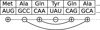
Figure 1. In the calculation of the CII each codon has an associated binary variable. Synonymous codons interact via the information theoretic part of the Hamiltonian (solid lines), nearest neighbour sites interact via the Ising interaction (dashed line).
Download figure:
Standard image High-resolution image2.1. Maximum information
We first consider the special case of a protein of length L composed of only one amino acid type, which can be translated by K different codons [34]; the generalization to the full set of amino acids is described below. The sequence {c1...,cL}, ci = 1,...,K is given, where ci is the ith codon. We associate a binary variable si =± 1 (i.e. a spin variable, rather than a bit ({0,1}) variable) to each site of the sequence; this spin variable identifies the class each codon is assigned to.
Let pc|s be the probability for the codon c to be used on a site with spin s. A priori, the only information available is that an amino acid can be encoded by any of its possible codons. This state of ignorance is described by the choice of a uniform prior distribution for the probabilities of the parameters pc|s, with the normalization ensured by a δ function
For any assignment  of the spins, the statistical information contained in the sequences is encoded in the codon counts
  , i.e. the number of times codon c is used on a site with spin s. The probability of observing
  is modelled using a product of two multinomial distributions

where  and obviously N+ + N− = L.
Using the Bayes formula P(θ|x) ∝ P(x|θ)P0(θ), we obtain the posterior distribution

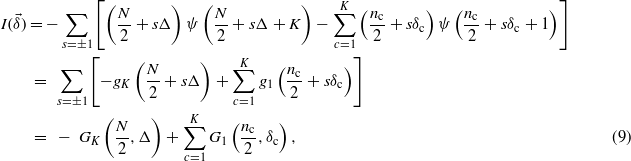
An important quantity that can be derived from the prior and the posterior is how much information is gained by observing the codon frequencies. This quantity is the symmetrized Kullback–Leibler divergence between the two distributions
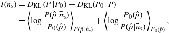
where the averages are performed with respect to the posterior, equation (3), and the prior, equation (1), respectively. The integration can be performed analytically and leads to

where ψ(x) is the digamma function.
The generalization to the whole set of amino acids is simply the sum of the  for each amino acid

where Ka is the number of codons encoding for the amino acid a, ns,a(ca) is the number of times a spin s is associated to the codon ca of the amino acid a and  .
.
To extract as much information as possible from the codon counts we have to maximize equation (5). However, the contributions of different amino acids are independent and each amino acid sector is invariant under a spin flip. Therefore, the minima of equation (5) are highly degenerate. Moreover, the amino acids with only one codon, methionine and tryptophan, do not contribute to equation (5).
These issues can be cured observing that the previous derivation does not use any information about how the codons are arranged along the sequence. Therefore, information carried by the codon order can be used to weight the minima of equation (5).
2.2. Codon spatial organization
In order to remove the degeneracy, we add to equation (5) an interaction between nearest neighbour spins that favours their alignment. This coupling is also consistent with the observation of the existence of a 'codon pair bias' [35, 36]. We thus define the cost function
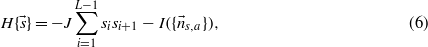
where J is a parameter to be tuned which accounts for the degree of spatial homogeneity of the sequence. In statistical physics terms, equation (6) can be regarded as the Hamiltonian of a spin system that, besides the 1D Ising interaction J, also has a long range interaction I as shown in figure 1.4 This analogy makes it possible to apply techniques used to study spin systems in statistical physics to the present model.
We are interested in the spin arrangements minimizing the Hamiltonian (6), given the codon sequence. Numerically, energy minimization was performed by simulated annealing Monte Carlo [37]. When the states of minimal H were found to be degenerate, an average over all of them was considered.
The optimization of the cost function H is carried out simultaneously on a pool of genes of the same organism, but clearly the nearest neighbour interaction is defined only for neighbouring codons within the same gene.
We define the local codon information index as the magnetization at site i on the transcript g, i.e. the thermodynamic average of the spin at site i

(an example is given in figure 2), and the codon information index of the gene g as the average of the local cII on the gene codons
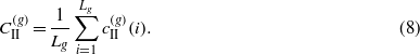

Figure 2. Local cII, as in equation (7), for the first 100 codons of the TFC3/YAL001C gene.
Download figure:
Standard image High-resolution image3. Phase diagram of the Hamiltonian (6)
In this section we characterize the properties of H in equation (5) and its minima. We will also prove the existence of a phase transition in temperature at J = 0. Finally, we will describe the effect of the nearest neighbour interaction.
3.1. Maximum of equation (5)
As a first step in the characterization of (5), we want to show that each term of the form (4) has a minimum and is convex. Let us rewrite (4) setting n±(c) = n(c)/2 ± δc, δc∈[ − n(c)/2;n(c)/2] and Δ = ∑cδc
where gi(x) = x ψ(x + i) and Gi(n,x) = gi(n + x) + gi(n − x).
We observe that I is symmetric with respect to a transformation  . Since gi(x) is continuous and differentiable in the domain, the derivative must be zero in
  . This point corresponds to a uniformly distributed posterior and, since I is computed as the KL divergence of the posterior from a uniform prior (which is a non-negative quantity and is zero iff the two distributions are equal), it is an absolute minimum. It is the only critical point since the system of equations

has the δi = 0 solution only, observing that  .
.
This implies that the maxima must reside on the boundary. Repeating the argument on the boundary faces, we end up concluding that the maxima must lie on the boundary vertices, i.e. the points such that  . On these points I becomes

The function is now only dependent on Δ and observing again that it is symmetric and concave we see that there is a maximum in Δ = 0.
The maximum is thus obtained on the vertices which minimize the difference |N+ − N−| (e.g., for four codons with {n(c)} = (5,3,4,2) the maximum is obtained for (+, − , − , + ) or (−, + , + , − ), since I is symmetric under a global spin flip). This is an instance of the number partition problem which belongs to the NP-complete class. However, we are dealing with sets which contain at most six elements.
Considering the full set of amino acids, we can finally ask how many states have the same  . Using the fact that the contribution for each amino acid is invariant under a spin flip and that the amino acids with one codon only are not considered, there are at least 218 states in addition to the trivial degeneracy coming from the amino acids methionine and tryptophan which do not contribute to (5).
3.2. Phase transition in temperature at J = 0
It is possible to analytically work out the thermodynamics of equation (6) at J = 0. At high temperatures we expect a disordered paramagnetic phase, while at low temperatures the system falls into one of its many minima, which correspond to the maxima of equation (5) described in the previous section. Here we prove that a phase transition exists by showing that the concavity of the free energy changes sign at a critical temperature Tc in the large nc limit.
At J = 0 we can easily compute the entropy of a state specified by  . The number of different configurations is simply the number of permutations of nc elements, given that the n+(c) and n−(c) are equivalent. The entropy is thus the logarithm of the product of binomials

and we can easily write the free energy F = H − TS,

At high temperature the thermodynamics of the system is governed by the entropic term which has a minimum at  (paramagnetic phase).
To prove that this minimum becomes repulsive at a critical temperature we study the concavity of the free energy. Taking the second derivatives gives
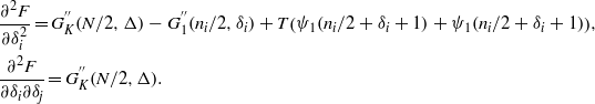
At high temperature we expect that |δi| ≪ ni. Expanding in large  , we find
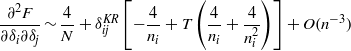
which can be written as  , where both ai =− 4(1 + T + T/ni)/ni and b = 4/N are independent of δi up to terms of order
  .
.
The free energy F is convex (concave) if the Hessian matrix is positive (negative) definite, i.e. if each eigenvalue is positive (negative). Its characteristic polynomial can be easily computed using the Sylvester's determinant theorem and reads as
Using some combinatorics, we obtain
with the convention α0 = 1. If  we immediately see that each coefficient is positive and thus the Hessian is positive definite, while if
  the Hessian is negatively defined because of the Descartes rule of signs5. At
  the free energy becomes convex and the ground state moves discontinuously far from the paramagnetic (
 ) state.
The order parameter which captures this phase transition is the codon coherence
where the sum is intended on every codon except methionine and tryptophan and the thermodynamic average is performed at temperature T. This parameter is small in the paramagnetic phase (which has 2δc = n+(c) − n−(c) = o(nc)) while it is one in the partitioning phase. Its plot is given in figure 3: the phase transition at T = 1 is evident, albeit smoothed out due to finite size effects.
3.3. Effects of the nearest neighbour interaction: J > 0
The introduction of the nearest neighbour interaction makes the analytical treatment much more difficult. Nevertheless, we expect that the phase transition will become smoother and smoother as J is raised, since the Ising model in 1D does not exhibit any phase transition. This observation is numerically tested in figure 3, where the profiles of ϕJ(T) are plotted for increasing J.
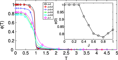
Figure 3. Codon coherence ϕJ(T) as a function of the temperature for increasing J and codon coherence at T = 0 (inset). As the nearest neighbour interaction is turned on, the phase transition becomes smoother. At T = 0, the codon coherence is preserved up to a critical value of J ∼ 0.3.
Download figure:
Standard image High-resolution imageThe T > 1 behaviour is easily understandable by observing that in the paramagnetic phase (δc ≪ nc) the information theoretical part of the Hamiltonian is flat around  in the large nc limit. We expect the high temperature (T > 1) behaviour to be dominated by the magnetic field and the nearest neighbour interaction terms: excluding the information theoretical part, the Hamiltonian reduces to the Ising model one,
  . Thus, the thermodynamics at T > 1 should be described by the phenomenology of the Ising model.
To check this hypothesis, we numerically computed the magnetization for the Hamiltonian (6)
as well as, analytically, the magnetization for the Ising model,
These quantities are plotted in figure 4, where is clearly shown that the Ising model correctly describes the T > 1 behaviour of (6).
We introduced the nearest neighbour interaction to weight the many minima of the information theoretical part of the Hamiltonian and to extract information from the spatial arrangement of the codons. Observing the inset of figure 3, we see that at J > 0.3 the codon coherence at T = 0 is lost. This means that the same codon is assigned a different cII on different positions. Since there is no a priori biological reason for this differentiation, we restrict the admissible J to those such that ϕJ(0) = 1. Moreover, since we want to maximize the information extracted from the spatial arrangement of the codons, we fix J as the maximum value such that ϕJ(0) = 1. Interestingly, we find that for this value of J the correlation of  with the tAI exhibits a maximum.
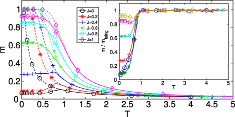
Figure 4. Solid lines: numerically computed magnetization as a function of temperature (equation (15)). Dashed lines: analytically computed magnetization of the Ising model in 1D (equation (16)). The inset shows the ratio m/mIsing. The magnetization for T > 1 is correctly described by the Ising model, and as J is raised the behaviour at T < 1 becomes more and more similar to that of the Ising model.
Download figure:
Standard image High-resolution image4. Analysis of the CII
4.1. CII correlates with protein and mRNA abundance
We computed the CII for a set of 3371 transcripts of S. cerevisiae and compared it with the logarithms of the measured protein [38] and mRNA [39] abundances, finding a significant correlation (C ≃ 0.60 and C ≃ 0.69 for proteins and mRNAs, respectively, figure 5).

Figure 5. The CII correlates with the logarithms of protein abundance (left) and mRNA abundance (right). The correlation is most evident for the most abundant half of the set (insets).
Download figure:
Standard image High-resolution imageIndeed, computing the same quantities for the half of the set comprising the most abundant proteins and mRNAs we observe a sharp increase in the correlation coefficients C ≃ 0.70 and C ≃ 0.79 for proteins and mRNAs, respectively.
4.2. CII correlates with tAI
A common method to address the translational efficiency of a gene is given by the tRNA adaptation index (tAI) [33], defined as
where wci is the weight associated to the cith codon in the gene g. These wc are defined as
where ni is the number of tRNA isoacceptors recognizing codon i, tGCNij is the number of the jth tRNA recognizing codon i and sij gauges the efficiency of codon–anticodon coupling. The sij are then optimized to maximize the correlation with protein abundance. The computation of this index requires information about two of the most influential factors affecting translation efficiency, namely tRNA abundance (tRNA copy number is highly correlated to tRNA abundance [40]) and codon coupling efficiency.
Computing the tAI for the same 3371 transcripts and comparing it with the CII we observe an extremely high correlation (ρ ∼ 0.93, see figure 7). We thus are able to reproduce all the results obtained from the tAI without needing any additional information beyond the codon sequences and without any parameter optimization: the CII depends only upon the parameter J which can be fixed from thermodynamics considerations, as explained in section 3.3.
The tAI is known to correlate well with protein abundance (ρ ≃ 0.61) and mRNA abundance (ρ ≃ 0.70), see figure 6. Moreover, also in this case the correlation improves for the most abundant proteins (ρ ≃ 0.70) and mRNAs (ρ ≃ 0.77) but to a significantly smaller extent with respect to the CII case.
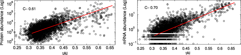
Figure 6. The tAI is highly correlated with protein (left) and mRNA (right) abundance.
Download figure:
Standard image High-resolution image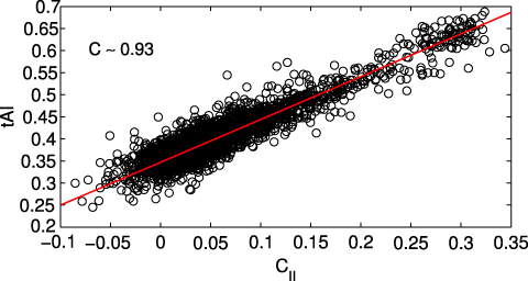
Figure 7. The CII is highly correlated with the tAI.
Download figure:
Standard image High-resolution imageAnother quantity usually taken into consideration in this kind of study is protein half-life. We computed correlations among all these quantities; the results are summarized in table 1. Between parentheses are the correlations computed for the 1600 most abundant proteins and mRNAs. All these values are statistically significant (P-value ∼10−9 at most). Those involving CII, tAI, protein and mRNA abundance are highly significant (P-value <10−20).
Table 1. Pearson correlation coefficients between numerical and experimental quantities. The values between parentheses, when present, refer to correlations computed for the most abundant half of the set.
| CII | tAI | Protein levels (log) | Half-life (log) | mRNA levels (log) | |
|---|---|---|---|---|---|
| CII | 1 | 0.93 | 0.60 (0.70) | 0.18 | 0.69 (0.79) |
| tAI | 1 | 0.61 (0.68) | 0.20 | 0.70 (0.77) | |
| Abundance (log) | 1 | 0.30 | 0.60 | ||
| Half-life (log) | 1 | 0.22 |
It has been suggested that the correlation between the CII and the mRNA levels can be caused by evolutionary forces acting more effectively on highly expressed genes [22], as beneficial codon substitutions are more likely to be fixed on these genes because the gain in fitness is likely to be higher, although a fully causal relationship can be more complicated and involve other determinants [11, 10].
4.3. Average CII profile along the proteins
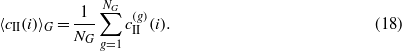
In the previous sections we analysed the properties of the global CII value for whole genes, but the cII(i) gives another local layer of information. We thus ask whether the local cII(i) can be interpreted as a local measure of translational optimality. Unfortunately too few data exist to confirm or falsify this hypothesis, but we can explore whether a common behaviour at the beginning of the transcripts exists. Similarly to the case of the tAI [29], it is possible to compute the average of the  across the transcripts,
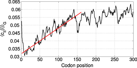
The plot in figure 8 reveals the presence of a 'ramp' roughly 120 codons long followed by a plateau.
Figure 8. Local cII averaged along the proteins, as in equation (18). The straight line is a guide for the eye.
Download figure:
Standard image High-resolution image
This result is consistent with the findings in [29] for the tAI, where this procedure reveals a signal at the beginning of the transcript: the average local tAI has a minimum at the beginning of the sequence and rises up to the average value in ∼100 codons. Since the authors claim that the tAI carries information about codon translational efficiency, they hypothesize that this feature helps translation stabilization by avoiding ribosome jamming.
5. Conclusions
In this work we have introduced the codon information index (CII) as a measure of the amount of information stored in mRNA sequences through the codon bias. We have shown that CII can capture at least as much complexity as previously introduced codon bias indices, but its computation does not require additional data beyond transcript sequences. In order to calculate the CII we do not make any assumption on the origins and roles of the codon bias, but quantify the amount of information associated with it in an unbiased manner, with a procedure that enables us to fully quantify the amount of such information.
We calculated the CII for a set of over 3000 yeast transcripts and found values highly correlated with the tAI scores, as well as with experimentally derived protein and mRNA abundances. Furthermore, we were able to reproduce the result that the first 70–100 codons are, on average, translated with low efficiency, a feature which is thought to help translational stabilization [29].
We anticipate that by using the CII it will be possible to investigate open questions about the role of the codon bias in optimizing translational efficiency, improving codon reading accuracy, and minimizing the risk of misfolding and aggregation.
Data sets
The set of RNA transcripts for S. Cerevisiae was downloaded from [41]. Protein half-lives were extracted from [42]. Protein and mRNA abundances were found in [39, 43]. Protein abundances were found in [44, 38].
Source code and details of the algorithm
The thermodynamic averages (and thus the CII) were computed using a Monte Carlo algorithm implemented with simulated annealing [37] and frequent reannealings: the temperature is a function of the simulation time and is slowly lowered. Provided that the cooling schedule is sufficiently slow, this method is guaranteed to sample the whole space, a vital feature if the free energy landscape is rough (meaning that the Hamiltonian has many metastable states).
The algorithm run time for the set of 3371 proteins was of the order of 1 day on a dual core workstation. The algorithm is massively parallelizable. A major speedup was obtained by observing that the energy differences of the information theoretical part of the Hamiltonian (6) (which are required in the Monte Carlo step) can be efficiently and locally computed using the properties of the digamma function. The code is available at the web page www-vendruscolo.ch.cam.ac.uk/CII/index.php.
Acknowledgments
Work partially supported by the GDRE 224 GREFI MEFI, CNRS-INdAM.
Footnotes
- 4
The Hamiltonian (6) is invariant under a global spin flip, thus the average magnetization would be zero. To break this symmetry it is sufficient to add a term Hh = h∑isi, which favours the configuration aligned with the external field h. The field h will be taken vanishingly small ideally, very small in practice.
- 5
The Descartes rule of signs states that the number of positive roots of a polynomial (known to have all real roots, like in this case, since we are computing the eigenvalues of a symmetric matrix) is equal to the number of sign differences between consecutive non-zero coefficients.