


Abstract
Alfvén Eigenmodes-driven fast-ion flows have been measured for the first time at the ASDEX Upgrade tokamak using an imaging neutral particle analyzer. The flow is such that particles are expelled from the mode location, losing energy as they move outwards. This flow aligns well with the projection of the lines of constant magnetic moment and constant E' ( , with E being the particle energy,
  the mode frequency and toroidal number and Pφ the toroidal canonical angular momentum). The observed redistributions are consistent with full-orbit simulations performed with the ASCOT5 code, using the mode structure predicted by the linear gyro-kinetic code LIGKA.
Export citation and abstract BibTeX RIS

Original content from this work may be used under the terms of the Creative Commons Attribution 4.0 license. Any further distribution of this work must maintain attribution to the author(s) and the title of the work, journal citation and DOI.
1. Introduction
In future fusion reactors, suprathermal particles (fast ions, FI) will play a key role in fusion power generation as they are an important source of energy (heating) and momentum (current drive) [1–3]. A poor confinement of these ions will lead to a decrease in reactor performance, and, if localized and intense, to damage in the first wall components [4, 5].
Understanding the mechanisms behind the suprathermal particle transport and losses is capital for achieving a future fusion power plant. One of the main observed causes for this particle transport and eventual loss is their interaction with a wide range of magnetic fluctuations, either intrinsic to the plasma, like neoclassical tearing modes (NTMs) [6, 7], fishbones [8–10] or Alfven eigenmodes [11–17]; or externally applied perturbations [18–21].
Previous studies in the ASDEX Upgrade (AUG) tokamak made extensive use of the fast-ion loss detectors (FILDs) [4, 6, 7, 11, 12, 14, 21–24] and fast-ion D-alpha (FIDA) and neutron diagnostics [25, 26] to study transport and losses caused by magneto-hydrodynamics (MHDs) perturbations. However, the FILD diagnostic is limited to the lost portion of the phase-space, while FIDA integrates over large regions of it, so the local interactions in phase space of FIs with the magnetic fluctuations cannot be fully explored. This investigation is essential to validate predictive modeling, which is key for the development of future actuators and control techniques. In this regard, the imaging neutral particle analyzer (INPA) [27–30] capabilities of measuring simultaneously energy and radial position of FIs in a narrow pitch range are a major advance. The visualization of the flows induced by reversed-shear Alfvén eigenmodes was carried out for the first time at the DIII-D tokamak [31–33]. These flows were also successfully compared against numerical simulations [34]. Here the first visualization of the fast-ion flows under the effect of toroidal Alfvén eigenmodes (TAEs) at the AUG tokamak is discussed.
This article is structured as follow: section 2 introduces in details the diagnostic setup. In section 3 the experiment results are presented while section 4 deal with the modeling of the observed transport.
2. Diagnostic setup
The INPA diagnostic measures fast neutrals produced in charge-exchange (CX) reactions between FIs and neutrals injected by a neutral beam injector (NBI). To this end, the CX neutrals are ionized by an ultra-thin carbon foil (20 nm) and deflected into a scintillator by the local magnetic field, as can be seen in figure 1 of [29]. The strike position on the scintillator, observed by a mega-pixel camera, allows for the reconstruction of energy and radial position of the FIs in the plasma [27, 29]. The AUG system covers from major radius R = 1.55 m (mid-plasma in the high-field side) all the way to the last closed flux surface on the low-field side (LFS), with a resolution of 7 cm and 9 keV, for full NBI energy deuterium ions [30]. The AUG INPA is only sensitive to passing ions, and explores a pitch ( , being
  the projection of the velocity along the magnetic field, which is directed in the opposite direction with respect to the plasma current at the AUG tokamak) near 0.55 in the core and 0.70 near the plasma edge. This pitch profile, calculated for discharge #41090, can be seen in figure 1, together with the fast-ion distribution calculated with the TRANSP code [35]. Full details of the diagnostic design, installation, validation and instrument functions can be found at [29, 30, 36, 37].
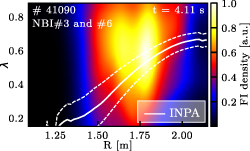
Figure 1. Fast-ion distribution calculated with TRANSP for the discharge #41090 at time 4.11 s. The distribution function was integrated in energy and z so just R and λ remain as variables. The central pitch explored by the INPA in each radial position is presented in white, the dashed lines represent the limits of the explored pitch in each radial position.
Download figure:
Standard image High-resolution image3. Experimental fast-ion redistribution
The studied scenario corresponds to an H-mode plasma with toroidal magnetic field on-axis of  T, a plasma current of
  kA, a
kA, a  (
( , being βt
the ratio of plasma pressure to toroidal magnetic pressure, and a the plasma minor radius), a core electron collisionality [38]
, being βt
the ratio of plasma pressure to toroidal magnetic pressure, and a the plasma minor radius), a core electron collisionality [38]  , and a core safety factor of
  ; following well-established fast-ion scenarios in the AUG tokamak [21, 39]. The temporal evolution of this discharge in the time range of interest can be found in figure 2. 2.5 MW of steady off-axis NBI and 2.5 MW of ion cyclotron resonance heating (ICRH) are applied to generate a large ratio, of energetic particle beta,
  ,
,  , to the thermal plasma one,
  ,
,  , of the order of 1. This is depicted in figure 2(b), where the fast-ion stored energy is shown together with the thermal stored energy. The used ICRH frequency is 36.5 MHz, which at the experiment magnetic field corresponds to the cyclotron frequency of H at R = 1.72 m. On top of this, 40 ms on-axis NBI blips (NBI#3) are added for diagnostic purposes. Despite this large input power, the electron temperature remains low (below 2 keV) due to the large radiated power, also shown in figure 2(b). The off-axis NBI source, NBI#6, was tilted to the maximal off-axis injection angle, maximizing the spatial gradient of the FI distribution, and hence achieving a stronger drive for the modes [40, 41]. Up to t = 4.2 s, during each beam blip, the plasma density peaks up to the same values (near
  at the core), while the temperature is gradually changing from blip to blip but less than 10% in the time range. This small increase should not have any impact on the INPA sensitivity [37]. Only a small increment in the INPA signal at the plasma core is expected, as predicted from the increase in the slowing-down time due to the electron temperature raise.
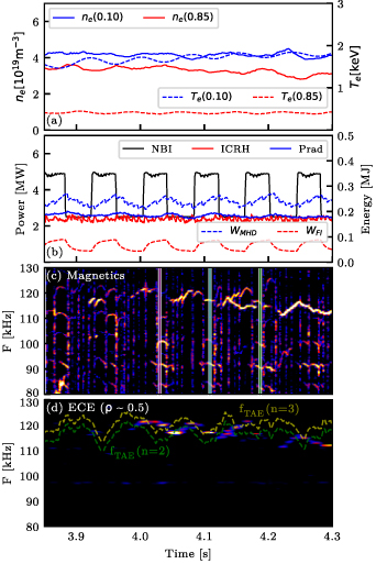
Figure 2. Evolution of plasma parameters for #41090 near t = 4.0 s. (a) Electron density (left axis) and temperature (right axis). (b) Injected and radiated power (left axis), stored energy (right axis). (c) Spectrogram from a magnetic coil, B31-14, in the LFS. The vertical lines represent the time points selected for the comparison of INPA signals. (d) Spectrogram from an electron cyclotron emission (ECE) channel near  ; the analytic frequencies (Doppler shifted) for the center of the TAE gap are plotted in dashed lines.
Download figure:
Standard image High-resolution imageFigure 2(c) shows the spectrogram from a coil located in the LFS while figure 2(d) shows the spectrogram associated with temperature fluctuations near mid-plasma, as measured by the ECE diagnostic. On both diagnostics, fluctuations in the frequency range of TAE can be observed. Under the effect of these modes, neoclassical predictions do not hold, as FIs interact with the TAEs and are redistributed [11, 21]. To visualize this particle transport caused by the TAE, two frames measured by the INPA diagnostic are compared: one without significant TAE activity (highlighted in magenta in figure 2(c)) and a second one with a large amplitude of the TAE, in a subsequent blip. The differences in the signal will correspond to the differences in the fast-ion distribution function, as the density profile is similar among them and hence, the INPA sensitivity will be equivalent [37].
Two groups of TAEs can be observed, the ones destabilized by NBI#3 (f < 110 kHz), which appear only when NBI#3 is activated; and the ones driven by NBI#6 and ICRH ( kHz), which are present even in the absence of NBI#3. The focus will be put in the modes at around 120 kHz, which are present throughout the whole time range.
The magnetic field line displacement, ξ, caused by the TAE mode can be extracted from the measurements of the perturbed electron temperature observed by an electron-cyclotron-emission radiometer thanks to the relation [42]:
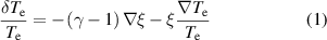
where  stands for the electron temperature and γ is the ratio of specific heats [43]. Neglecting the compressional term,
  , due to the shear nature of the TAE mode, the radial displacement can be obtained as:
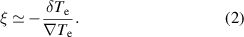
This radial displacement is shown in figure 3. Two groups of peaks can be observed, one near the plasma core, centered at about  , and another one off-axis, near
  for the n = 3 mode and near 0.40 for the n = 2 mode. The toroidal mode number n was obtained from the phase correlations of the set of toroidally distributed magnetic coils in the AUG tokamak.
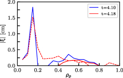
Figure 3. Field line radial displacement caused by the TAE. Dashed line corresponds to n = 2 modes while solid line corresponds to the n = 3 component.
Download figure:
Standard image High-resolution imageThe INPA signals at the time points represented in figure 2(c) are plotted in figures 4(a)–(c). Subplots (d) and (g) show the electron density and temperature profiles, respectively. The differences in the signal (FI population) between the frames at t = 4.10 s (strong modes near 115 kHz, cyan in figure 2(c)) and t = 4.02 (no modes at 115 kHz, magenta in figure 2(c)) are depicted in subplot (e). Subplot (f) shows the equivalent difference but for the frame at t = 4.18 s. There is a significant decrease (outflow) in the signal when comparing the two first frames, corresponding to a decrease in the fast-ion density within the radial range 1.7–1.8 m, where the larger mode peak is located (ρ < 0.2). This decrease (outflow), of a few percent compared to the maximum signal, comes together with an increase (inflow) in the radial range above 1.8 m, at smaller energies. These local outflow and inflow of the FI distribution can be understood as a sign of TAE-induced particle transport. To understand the connection of these areas of inflow and outflow of the fast-ion density, the flow streamlines [31, 33] are plotted with dashed lines in figures 4(e) and (f). These streamlines are the intersection of the surfaces of constant µ and E' ( , with E being the particle energy,
  the mode frequency and toroidal number and Pφ
the toroidal canonical angular momentum), the two conserved quantities in the interaction between the FI and the TAE [44]. Only the portion of the stream line which lies inside the pitch range explored by the INPA diagnostic is plotted. The reference signal, and signal differences, interpolated along those lines are plotted in figure 5. It can be observed how the decrease (outflow) of the signal (FI population) coincides with the areas where there is a large gradient on the FI population along the stream line. Hence, the mode is causing a flattening of the FI distribution gradient along the flow line.
the mode frequency and toroidal number and Pφ
the toroidal canonical angular momentum), the two conserved quantities in the interaction between the FI and the TAE [44]. Only the portion of the stream line which lies inside the pitch range explored by the INPA diagnostic is plotted. The reference signal, and signal differences, interpolated along those lines are plotted in figure 5. It can be observed how the decrease (outflow) of the signal (FI population) coincides with the areas where there is a large gradient on the FI population along the stream line. Hence, the mode is causing a flattening of the FI distribution gradient along the flow line.

Figure 4. Differences in the INPA signal. First column (a)–(c): raw INPA signal for each time point. (d) and (g) Density and temperature profiles. (e)–(f) Differences in INPA signal between the given time and the reference frame at t = 4.02 s. (h)–(i) Differences in the synthetic signals. The FI distribution was taken from a time evolving TRANSP simulation while the INPA sensitivity was taken at the reference frame. The vertical dashed lines indicate the position of the magnetic axis.
Download figure:
Standard image High-resolution image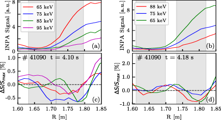
Figure 5. Interpolation of the INPA signal along the stream lines. (a) INPA signal at the reference time point, t = 4.02 s interpolated along the stream lines showed in figure 4(e). (b) Equivalent for the stream lines shown at figure 4(f). The energy in the legend indicates the energy of the stream line at R = 1.8 m. (c) Changes in the INPA signal (FI distribution) along the stream lines when comparing t = 4.10 s (strong n = 3 TAE) and t = 4.02 s (reference), normalized to the signal maximum at the reference frame. (d) Equivalent to (c) but for t = 4.18 s (strong n = 3 and n = 2 modes). Shaded areas represent the mode locations.
Download figure:
Standard image High-resolution imageThis behavior is opposite to the neoclassical prediction. The predicted changes in the INPA signal are depicted in figures 4(h) and (i). This is calculated with the workflow detailed in [29]: TRANSP [35] simulations are used to predict the neoclassical fast-ion distribution function, FIDASIM [45, 46] simulations to model the CX influx at the detector entrance, and an upgraded version of FILDSIM [37] to track the markers until the scintillator plate. The comparison between the energy-integrated INPA measurement and the neoclassical simulation is depicted in figure 6. A significant depletion of the INPA signal (of the order of 5%) is observed close to the magnetic axis, where the inner mode peak is located, together with an increase of almost 10% in the off-axis region.
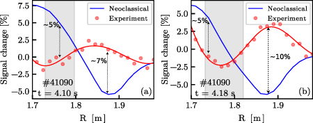
Figure 6. Comparison of experimental and neoclassical energy-integrated radial relative changes. The shaded areas represent the mode location. (a) Comparison for time = 4.10 s. (b) Comparison for t = 4.18 s. In both cases, the solid red line represents a smoothing cubic interpolation performed to ease the comparison of the experimental data with the neoclassical calculations.
Download figure:
Standard image High-resolution image4. Modeling of the fast-ion redistribution
In order to mimic the FI transport observed in the experiment, the mode structure is simulated with the LIGKA code [47–50] and inserted in the full-orbit ASCOT5 code [51], where markers from the distribution function calculated by TRANSP were followed. No Coulomb collisions are included in ASCOT5, in order to isolate the effect of the MHD modes.
The shear-Alfvén wave continuum calculated with LIGKA together with the experimental mode frequency are shown in figure 7. The measured mode frequency was Doppler shifted taking into account the rotation frequency at ρ = 0.15,  kHz to obtain the mode frequency in the plasma frame.
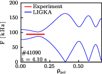
Figure 7. SAW continuum calculated with the LIGKA code. In red, the experimentally determined mode frequency. The radial extension of the red line corresponds to the mode extension.
Download figure:
Standard image High-resolution imageThe amplitude of the mode electrostatic potential for a poloidal mode number larger than zero,  , is obtained from the radial displacement using the relation [52]:
where r is the minor radius, defined as the distance along the LFS mid plane between the magnetic axis and a given flux surface. The radial velocity,  , can be obtained from the radial mode displacement as:

where ω is the mode frequency. With this, the amplitude of the electrostatic potential becomes:
For the time t = 4.10 s, LIGKA finds a mode with  in the region near ρ = 0.15 while for the frame at t = 4.18 s, a mode with
  is found. Using the radial profiles depicted in figure 3 this translates into amplitudes of 200 V and 270 V, respectively. For the simulations, only the peaks of the innermost mode which have the larger observed radial displacement were used. Their structures can be seen in figure 8. Figure 8(a) shows the 2D mode structure while subplot (b) shows the comparison of the radial mode electrostatic potential as measured by the ECE and simulated by LIGKA at t = 4.10 s. Notice that, as LIGKA is a linear code, it does not provide the mode amplitude. The mode amplitude was scaled to match the measured potential. A perfect agreement in both mode location and width is found between LIGKA and the experiment. For the case of t = 4.18 s, the peak location is still well matched by LIGKA, although a small under-prediction in the mode width is found.
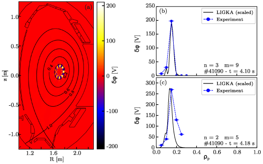
Figure 8. Comparison of simulated and measured mode structures. (a) 2D image of the electrostatic potential simulated with LIGKA. (b) Radial profile of the measured electrostatic potential (only the peak of the larger radial displace is included) and the scaled LIGKA simulation. #41090, t = 4.10 s. (c) Similar to (b) but for the timepoint 4.18 s.
Download figure:
Standard image High-resolution imageThe computed redistributed fast-ion phase space is then fed to the INPA synthetic diagnostic, enabling a direct comparison to the experimental signals. This comparison can be seen in figure 9. Subplots (a)–(b) show the differences registered at the INPA signal. The differences predicted when the inner mode peak obtained with LIGKA is fed into ASCOT are depicted in subplots (c)–(d). A good agreement is found among them. Particles near the magnetic axis, represented with the vertical blue line, are expelled towards larger radii and smaller energies, following the conservation of E'. Note that the off-axis region between 1.8 and 1.9 m is populated in the experiment by both the on-axis mode redistributing particles outwards and the off-axis mode redistributing them inwards while in the simulation only the inner mode is present, so this off-axis increase is hardly noticed. The agreement is better seen when comparing the local signal changes in radius, integrating along energy as done previously in figure 6 for the neoclassical simulation. This integration is shown in figure 10. The radial region where the depletion takes place is well captured by the workflow, apart from a small shift of a couple of cm, in the range of the INPA radial resolution (4 cm) and the used grid size for the calculation of the synthetic signal. The absolute level of the redistribution is also well in line with the measured redistribution.

Figure 9. Comparison of measured and simulated redistributions caused by TAEs. The first row shows the comparison for the case of t = 4.10 s. The second row shows the equivalent for t = 4.18 s. First column reproduces the experimental observation while the second column shows the ASCOT simulation. The dashed lines corresponds to the streaming lines while the shaded areas correspond to the mode location.
Download figure:
Standard image High-resolution image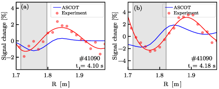
Figure 10. Comparison of experimental and synthetic energy-integrated radial relative changes. The shaded areas represent the mode location. (a) Comparison for time = 4.10 s. (b) Comparison for t = 4.18 s.
Download figure:
Standard image High-resolution image
5. Conclusions
The first visualization of the fast-ion phase space flow driven by TAEs at the AUG tokamak with Ion Cyclotron Heating has been measured with the INPA diagnostic. It was verified that FIs lose energy as they are transported outwards by the mode, as expected from the E' conservation. The redistribution is such that the gradient of the distribution, along the flow lines, is reduced.
Modeling with the ASCOT code using the experimentally identified eigenfunctions from the LIGKA code agrees quantitatively with the observed redistribution caused by the mode near the core. The transport along the  stream line is well reproduced, demonstrating that linear simulations with a fixed Eigenmode structure suffice to understand the core redistribution caused by TAE.
Acknowledgments
This project received funding from the European Research Council (ERC) under the European Union's Horizon 2020 research and innovation program (Grant Agreement No. 805162) and the Spanish Ministerio de Ciencia, Innovación y Universidades (Grant No. FPU19/02486). J. Galdon-Quiroga acknowledges support by the European Union under the Marie Sklodowska Curie Grant Agreement No. 101069021. This work has been carried out within the framework of the EUROfusion Consortium, funded by the European Union via the Euratom Research and Training Programme (Grant Agreement No. 101052200—EUROfusion). Views and opinions expressed are however those of the author(s) only and do not necessarily reflect those of the European Union or the European Commission. Neither the European Union nor the European Commission can be held responsible for them.