


Abstract
A toroidal Alfvén eigenmode (TAE) has been observed to be driven by alpha particles in a JET deuterium-tritium internal transport barrier plasma. The observation occurred 50 ms after the removal of neutral beam heating (NBI). The mode is observed on magnetics, soft-xray, interferometry and reflectometry measurements. We present detailed stability calculations using a similar tool set validated during deuterium only discharges. These calculations strongly support the conclusion that the observed mode is a TAE, and that this mode was destabilized by alpha particles. Non-ideal effects from the bulk plasma are interpreted as responsible for suppressing the majority of TAEs which were also driven by alpha particles, but the modes that match the observations are predicted to be particularly weak for these non-ideal effects. This mode located far from the core on the outboard midplane is found to be driven by both trapped and passing particles despite alpha particles originating in the core.
Export citation and abstract BibTeX RIS

Original content from this work may be used under the terms of the Creative Commons Attribution 4.0 license. Any further distribution of this work must maintain attribution to the author(s) and the title of the work, journal citation and DOI.
1. Introduction
The recent JET deuterium-tritium (DT) experiments [1] provided a rare opportunity to observe megawatts of fusion power produced in a tokamak and the associated effects of alpha particles on the plasma stability. Although energetic particles introduced by external heating are ubiquitous in modern tokamaks, and their associated stability effects are observed routinely, they have important differences to alpha particles. Resonant kinetic instabilities obtain their free energy from the details of the fast ion velocity distribution, depending on both the magnitude and direction of the fast ion motion. In magnitude, very few modern tokamaks can confine MeV range particles and do not introduce them. In direction, neutral beam and ion cyclotron resonant heating (NBICRH) are very narrow in the space of trajectories that they populate, whereas alpha particles are emitted uniformly in pitch angle by the fusion reactions.
The toroidal Alfvén eigenmode (TAE) [2] is an important instability of concern for ITER [3] which is driven through the resonant wave-particle interactions with alpha particles [4, 5]. On JET, it is difficult to produce sufficient number of alpha particles to drive TAEs beyond the stabilizing effects of the bulk thermal and NBI population [6]. In order to optimize the chances of observing alpha driven TAEs in DT, an internal transport barrier (ITB) scenario at elevated safety factor  incorporating an 'afterglow' was developed for the 'ITER-like' Be/W wall (JET-ILW) [7]. To avoid the possible excitation of Alfvén Cascades, observed on the Tokamak Fusion Test Reactor (TFTR) [8], the
  profile during the high performance phase was designed to be monotonic. Extrapolations of TAE stability based on analysis of pure deuterium reference discharges [9] predicting 8 MW of DT fusion power resulted in sufficient alpha power for a single marginally unstable TAE towards the edge of the plasma.
A marginally unstable TAE has subsequently been observed in JET DT shot 99946 from the 2021 DTE2 campaign, carried out with Be/W wall. In this paper, we present detailed stability analysis of this pulse.
2. Theory
Alpha particles produced in DT fusion reactions have energies which can both heat the plasma and destabilize it. In an axisymmetric tokamak, they are confined to imaginary surfaces labelled by three invariants of motion: the energy  , the magnetic moment
  , and the toroidal canonical momentum
  . The toroidal canonical momentum is a combination of poloidal flux
  and toroidal velocity through the relation

The relative contribution of the two terms in  gives the deviation of the particle surfaces from the magnetic surfaces. In the case of trapped particles which have the largest deviation, the orbit width is approximately
  for ion Larmor radius
  elongation
  and inverse aspect ratio
  . For JET at elevated
  , the ratio of this width to minor radius approaches unity for an alpha particle, whereas for a thermal particle
  is much more justified. This has implications for the representation of the equilibrium and how the stability is analysed.
The DT ions and electrons in local thermal equilibrium constitute the bulk of the plasma energy and density, with aspects of the force balance and stability well modelled by magnetohydrodynamics (MHD). The toroidally symmetric equilibrium can be described as a fluid with the Grad-Shafranov equation
where the functions of poloidal flux  correspond to the pressure force
  and the covariant toroidal magnetic field
  . The representation of the equilibrium of the fast ions, which are not in local thermal equilibrium, depends on the details of their velocity distribution. If their energy content is comparable with that of the bulk plasma, then equilibrium reconstruction using the fluid model equation (2) will not capture all the forces present. For example, fast populations in general cannot be represented by an isotropic pressure. A satisfactory compromise commonly used for NBI force balance on JET is the fast pressure approximation [10] to include the fast particle forces in the Grad-Shafranov equation. The alpha stored energy on JET is of order a few percent of the thermal bulk and can be neglected in the equilibrium reconstruction, whereas the NBI energy is approximately 20% of the total energy content.
An important mode of oscillation in the bulk DT plasma is the TAE, which is a largely incompressible shear Alfvén wave at low values of  and conventional aspect ratio. Nonuniform magnetised plasma, as found in a tokamak, supports a continuum of singular Alfvén wave solutions
  for parallel wavenumber
  and Alfven speed
  , with geometrical effects opening gaps in the continuous spectrum. TAE solutions are discrete non-singular modes found within a spectral gap centred at
In ideal MHD, modes such as the TAE exhibit neither growth nor damping unless they are singular, so a purely thermal plasma does not drive TAEs. The so-called kinetic effects, which include finite ion Larmor radius, a finite parallel electric field, and wave-particle resonances, are not taken into account in the ideal MHD model [11]. While these effects are typically weak and do not significantly alter the mode frequency or spatial structure, they are essential in understanding mode damping in practical fusion experiments because the drive is also weak. The non-resonant kinetic effects modify the local dispersion relation [12] to

for ion Larmor radius  and resistive dissipation by electron collisions
  . This creates a coupling between the TAE and kinetic Alfvén wave which leads to radiative damping [13]. The relationship between parallel current and parallel electric field for the TAE can be modelled in MHD with a complex resistivity
  [14, 15]
The resonant kinetic effects take place when ions exhibit velocity components that match the phase velocities of the TAE. This resonance can occur for the tail of the nearly Maxwellian ion distribution in the bulk plasma during ion Landau damping, or for the fast particles associated with NBI or alpha heating. The equilibrium expressed in the kinetic picture is that of an equilibrium distribution function expressed in terms of constants of motion such as  where
where  is the sign of the velocity parallel to the equilibrium magnetic field.
Assuming the general form for the equilibrium distribution function, the linear wave-particle modification to the TAE growth rate is given by [16]
where  is toroidal mode number,
  and
and  are the bounce-averaged
  toroidal and poloidal frequencies of the particles, and
  is an integer that labels each Fourier component in the time varying wave-particle power transfer. The coupling coefficient
  can be computed from the work done on a particle over a bounce period divided by the energy in the wave. The sign of
  at each resonance governs whether the contribution from those resonant particles will be stabilizing or destabilizing. For resonant bulk thermal and NBI ions on JET there are resonances of sub-Alfvénic populations where energy gradients are stronger than radial gradients and
  , implying both populations are stabilizing, whereas for resonant alpha particles there are super Alfvénic particles with
  .
.
The resonance condition appearing in the denominator below  (equation (6)) is a function of the unperturbed orbit passing through
  . The Fourier amplitude of the orbit power transfer will vary with the integer
  , but some limiting cases can be identified. For example, a deeply passing orbit which is approximately bound to a magnetic flux surface will resonate strongest when
  for one of the TAE poloidal harmonics
  which translates to
  . The deviation of the orbit from flux surfaces distorts this simple picture and sideband resonances appear at
  . A complementary limiting case occurs for deeply trapped particles
  with sidebands
  . The power transfer between waves and alpha particles in JET could look significantly more complex than in a reactor because of the large deviation of alpha particle orbits. Large orbits increase the influence of
  sidebands, but also, populate the edge regions of high magnetic shear where TAEs have more poloidal harmonics
  . Such a dense spectrum of resonances could also be important for understanding anomalous alpha transport through the overlap of resonances.
In the following sections, we present the experimental observations of the JET-ILW ITB afterglow, the calculated fluid and fast particle equilibria, the stability analysis, and compare to observations.
3. Experimental observations
3.1. Overview of the JET ITB afterglow
The 50–50 DT ITB shot 99946 investigated in this paper is the highest performant version of the ITB afterglow developed for JET DT with Be/W wall [7]. The previous paper that we published, which focused on the validation of stability calculations, examined a similar DD scenario [9]. We summarize here the key features of the JET-ILW ITB scenario. These scenarios involve monotonic safety factor  low shear discharges with a vacuum magnetic field of 3.4 T and a plasma current of 2.5 MA, operating at elevated
  values greater than 1.5. The pulses are approximately 50:50 DT at the time of interest (
 dominated by high-Z metallic impurity), although equal concentrations of D and T is difficult to achieve and validate in the core for these short pulses at low density. NBI heating above 25 MW in JET with the ITER-like (metal) wall can lead to the formation of an ITB at the
  surface, with some sensitivity to timing and density, the latter being set as low as possible. Strong density and ion temperature peaking are a feature of this scenario which can result in ion/electron temperature ratios of around
  when the discharges are successful in producing an ITB. The ITB is obtained in order to achieve a high fusion performance thereby resulting in a significant alpha particle population.
Shot 99946 achieved a maximum 50:50 DT fusion power of  with core temperatures
 and core density
  achieved with the intermittent application of NBI at 29 MW, the intermittency coming from the unpredictable behaviour of the bank of 16 positive ion neutral injectors (PINIs) needing to deliver power simultaneously. Performance of the ITB scenario was sensitive to this intermittency as the ability to obtain an ITB at this power level was found to be marginal in DD and DT. Half the PINIs were injecting deuterium and the other half injecting tritium, with beam energies varying around approximately
  . The plasma parameters of electron density, electron temperature, ion temperature, and toroidal rotation were measured using various techniques. The electron density was measured using high time-resolution Thomson scattering (HRTS) [17] and LIDAR Thomson scattering [18]. The electron temperature was measured using HRTS and electron cyclotron emission (ECE) [19]. To measure both ion temperature and toroidal rotation, D and Ne charge exchange recombination spectroscopy (CXRS) [20] and x-ray crystal spectroscopy (XCS) [21] techniques were employed. The measured plasma profiles with major radius are presented in figure 1 for the time of maximum fusion power
  , along with examples of profile fits which are used in our analysis described later in this paper. The time evolution for pulse 99946 is given in figure 1, showing the ELM timing as detected by average inner divertor Be II photon flux. Deuterium pacing pellets fired at the maximum rate of 45 Hz were used to mitigate large type-I ELMs. Without this mitigation, large impurity influx of tungsten would follow a large ELM and result in radiative collapse of central electron temperature and disruption. No ICRH was applied, meaning that the only population of ions exceeding the Alfvén speed were produced in the fusion reaction. ICRH is believed to be an important factor in preventing core high Z impurity accumulation, so these pulses were designed to deliver their maximum fusion rate transiently and as early as possible before impurities led to degradation and destabilization of the plasma. To determine the optimal time to remove NBI heating, real-time control was utilized to detect the point of maximum neutron rate.
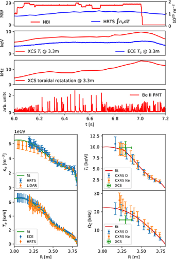
Figure 1. Plasma scenario for shot 99946. The time evolution (top) showing NBI power, line-integrated electron density, electron and ion temperature, toroidal rotation, and ELM timing. The radial profiles along plasma midplane from magnetic axis to outboard edge are given (bottom) for electron and ion temperature, toroidal rotation, and electron density. Fits to data used for analysis are also shown. The profiles shown are obtained at 7.0 s when the measured neutron rate was a maximum.
Download figure:
Standard image High-resolution image3.2. Mode observations
TAE stability extrapolations from DD [9] as well as past experience from TFTR [22] suggested that TAE modes if unstable could be difficult to observe on magnetics alone, particularly if destabilized in the core. A range of diagnostics were available to detect fluctuations in the plasma and associated density and field oscillations. Density fluctuations could be detected via reflectometry [23], interferometry [24] and soft-xray emission [25], the latter two being line integrated measurements.
Figure 2 presents the time evolution of neutron rate and input power for pulse 99946 along with the associated density fluctuation measurements. The graph illustrates a steady improvement in fusion power as heating is applied, with a notable enhancement commencing at 6.6 s, which coincides with the central ion temperature rising, deviating further from the steady electron temperature. At time of peak fusion power, 7.0 s, the NBI heating is removed, with a subsequent decay in neutron rate. Prominent in both the Fourier spectra in figure 2 are oscillations covering the full range of frequencies from 10 to 150 kHz. These features were absent from pure deuterium and pure tritium experiments conducted during the development of the DT scenario. Whilst these previous discharges did not have exactly the same NBI power and performance and cannot be said to be 'reference' discharges, the fact that these mode features were absent in dozens of similar discharges is interesting. However, it is revealing to compare these results to the spectrum obtained from magnetics in figure 3. Only a subset of these features are present in both spectra, and can be identified with toroidal mode numbers  . Using these modes observed on magnetics as reference, the additional modes in the soft-xray data appear to have frequency evolution corresponding to frequencies constructed by the sum or difference of these reference modes. This suggests that the signal may depend on the product of the linear modes, which could be a property of the plasma or the diagnostic's response to these modes. In either case, these prominent and apparently nonlinear features cannot be treated as eigenmodes from the linear plasma theory.
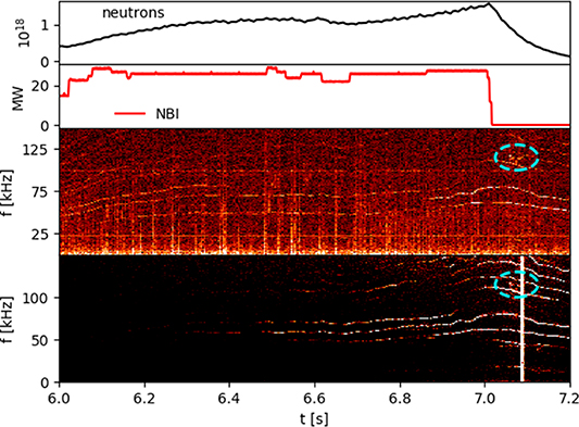
Figure 2. Mode observations during the afterglow in JET DT shot 99946. Fusion neutron rate (top), input NBI power (second), Fourier Spectra from interferometry (third) and soft-xray emission (bottom). TAE candidate appears in both spectra at 7.05 s with frequency 115 kHz (circled).
Download figure:
Standard image High-resolution image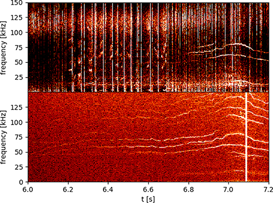
Figure 3. Spectra obtained from Mirnov coil (top) and soft-xray camera (below) for shot 99946. Nonlinear harmonics of low frequency oscillations are present on soft-xray data but not on magnetics.
Download figure:
Standard image High-resolution imageOnce the prominent long lived modes are discounted, the remaining feature evident in figure 2 is a faint oscillation at 115 kHz beginning at 7.05 s which is 50 ms after the removal of NBI heating. This feature is present in both spectra, suggesting the likely interpretation of a density oscillation in the plasma. The thermalization time [26] for the NBI is ∼140 ms, whereas for the alphas it is ∼230 ms. Crucially, this oscillation is also discernible on the spectrum obtained from a Mirnov coil, although faintly compared with other activity. Figure 4 shows a cross-correlation between soft-xray data and magnetics to improve the contrast. The appearance of the oscillation on magnetics is consistent with an electromagnetic mode of the plasma involving a magnetic perturbation. This faint mode was barely discernible on the magnetic probes so a measurement of toroidal phase shift, and therefore the toroidal mode number  , has not yet been successful.

Figure 4. Spectrum of the cross-correlation of phase (centre) between Mirnov coil data (top) and soft-xray data (bottom) for shot 99946.
Download figure:
Standard image High-resolution imageThe absence of toroidal mode number measurement presents a setback in two ways. Firstly, it makes it difficult to determine how the plasma rotation Doppler shifts the observed frequency in the laboratory frame for the mode. Secondly, it provides fewer constraints on linear stability calculations. However, the lack of Doppler shift information can be partially mitigated by observations of the mode localization with respect to the rotation profile. Rotation profiles were obtained CXRS when NBI was present, corroborated with a line-averaged XCS measurement near the core, the latter continued to be available after NBI was removed. Mode localization information was determined by reflectometry [27, 28], consisting of W-band and F-band X-mode correlation reflectometers with a pre-programmed frequency sweep. The frequency sweep allowed detection of density fluctuations with position that varied with the microwave frequency. Spectra were obtained simultaneously from two different frequency bands: the F-band (i.e.: 90–140 GHz) was probing the core ∼3.1 ± 0.1 m, and the W-band (75–110 GHz) was probing the edge ∼3.6 ± 0.1 m. The spectra obtained from reflectometry are presented in figure 5. The 115 kHz mode was observed only on the external measurements over a range of positions between 3.4 m–3.6 m  , and was simultaneously absent over the range 3.1 m–3.3 m
  . A nonlinear harmonic of a low frequency oscillation below the mode of interest is the only feature seen on the core measurement, and this can be easily identified in the spectra presented earlier in figure 2. CXRS rotation data at full power for this external region of the plasma gives the plasma toroidal rotation between 5 kHz at 3.8 m and 15 kHz at 3.5 m (figure 1).
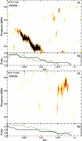
Figure 5. Reflectometry measurements of the density fluctuation spectrum for (a) with position scanning in time (b). At the time of interest, the F-band (top) was probing close to the core whilst the W-band (bottom) was probing closer to the edge. Two different estimates for radial cut-off are provided using different measurements of density. Obtained from JET shot 99946.
Download figure:
Standard image High-resolution imageHaving observed an electromagnetic mode at 115 kHz during the afterglow, lying outside the central ITB region that ends at 3.48 m, we now proceed to calculations of equilibrium and stability to help identify the mode as a TAE.
4. Calculations
4.1. Fluid equilibrium reconstruction
Equilibrium reconstruction on JET with the EFIT code typically requires internal measurements, particularly motional Stark effect (MSE), to accurately infer the safety factor  [29, 30]. The plasma pressure contribution to the Grad-Shafranov (equation (2)) is routinely available through temperature and density measurements, along with calculations of neutral beam pressure, however MSE is not available during the afterglow, and only available sporadically during the high-performance phase. This means that the magnetic pressure term
  is unconstrained, leading to large uncertainty in
  As in our previous study in DD plasmas [9], we constrained the plasma pressure in the reconstruction, but we have implemented tension splines to better capture the pedestal region. Also as in our previous work, we make use of the available MHD activity to identify the location of rational surfaces
  . Modes identified on the Mirnov array were analysed for toroidal phase to obtain toroidal mode number and then cross-correlated against electron cyclotron emission (ECE) to obtain position [31].
In practice, modes could be observed directly on the spectra obtained from a given ECE radial channel, with the strongest channel also easily obtained by inspection. Figure 6 contains an example spectrum from a single ECE channel which corresponds to radial location 3.25  0.02 m. Modes that were measured as n = 3 and n = 4 on the Mirnov array can be seen 7.0 s and 7.3 s respectively on the ECE channel. Given the low frequencies of the modes observed, it was assumed that modes were associated with rational surfaces
  . Many modes at low frequencies such as tearing modes, and beta-induced Alfvén eigenmodes satisfy this assumption. Poloidal mode number m in the ratio
  , although not measured, can be inferred by process of elimination given the location of other measurements required to give a smooth profile. The resulting MHD markers are summarized in table 1.
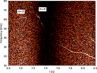
Figure 6. Spectrum obtained from a single ECE channel at R = 3.25 m. An n = 3 mode appears at 7.0 s, whereas an n = 4 mode appears at 7.3 s. Obtained from JET shot 99946.
Download figure:
Standard image High-resolution imageTable 1. Rational surfaces inferred from MHD markers used for equilibrium comparison. Obtained from JET shot 99946.

|

|

|

|

|
|---|---|---|---|---|
| 7.3 | 1 | 2/1 | 3.42 | 7.8 |
| 7.0 | 4 | 7/4 | 3.35 | 80 |
| 6.5 | 4 | 7/4 | 3.29 | 59 |
| 7.0 | 3 | 5/3 | 3.25 | 62.5 |
| 7.3 | 4 | 7/4 | 3.25 | 58 |
| 7.3 | 3 | 5/3 | 3.16 | 50 |
Tension splines are the standard way to parameterise the unknown poloidal flux functions in EFIT when constraints to pressure measurements are used. This is always subject to a regularisation condition to prevent over-fitting of the input pressure data. This is achieved in EFIT with a constraint that adjacent spline knot points should have some relationship which imposes spatial smoothing, with the weighting of this difference a tuneable numerical parameter. To decrease observed arbitrary oscillations in the inferred profiles, the relational constraint between the knot points was increased by a factor of 10 over values that are normally used. The safety factor at the magnetic axis was also constrained towards  such that
  was consistent with the measured MHD markers, since these individual measurements could not be directly included in the equilibrium constraints. The resulting equilibrium reconstruction of q-profile is presented in figure 7, along with an MSE reconstruction using the established JET settings. We can see that the standard MSE reconstruction intersects the measured MHD markers very well, despite being done for an earlier part of the discharge at
  . For the custom recipe involving q(0) constraint, the agreement at all three times is excellent, with the time of interest
  shown in the figure. This latter equilibrium is used for all the subsequent analysis presented below. The MSE profile was not used because, although it has broad agreement with the MHD markers, it did not have as detailed agreement as the custom reconstruction. Moreover, having been obtained 0.9 s earlier than the time of interest, there is no expectation that the q profile should remain constant on that timescale. It should be mentioned however that at
  , no MHD marker was available for the
  surface. It is quite possible that the location of the
  surface was unchanged from measurements at
  , also matching the MSE reconstruction at
  . If true, this would systematically shift possible TAE predictions on the outboard plane outwards by about
  cm. There is some suggestion of this shift when comparing mode locations to the MHD results below, but we have not contrived our equilibrium to accommodate this assumption.
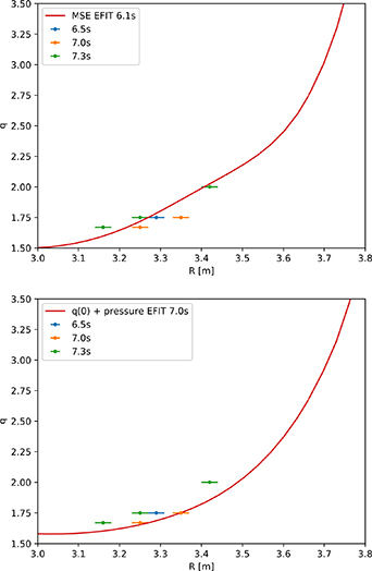
Figure 7. Reconstructed safety factor compared with MHD markers for standard MSE (top), and q(0) and pressure constrained (bottom) methods. Markers at three different times are presented in each plot. Obtained for JET shot 99946.
Download figure:
Standard image High-resolution image4.2. Incompressible linear stability
To identify if the candidate electromagnetic mode could be a TAE, we used the incompressible cold plasma model for the bulk plasma to identify the available TAE solutions for the reconstructed  profile. Our previous study in DD [9] demonstrated reproduction of the TAE frequencies within a few percent. We repeated the same procedure for 99946 at 7.05 s. The transformation of the equilibrium to the straight field line coordinate representation was performed with HELENA [32], then TAE solutions were found with the linear ideal incompressible eigenvalue solver MISHKA-1 [33]. As toroidal mode number measurements were not available for this faint mode, the range of
  used in the search needed to be constrained by other considerations. The hydrogen minority TAEs observed in previous DD studies were found to have toroidal mode numbers
  . The efficiency of wave particle interaction is generally optimal when the mode width is similar to the orbit width. Given that we expect the orbit width of alpha particles to be double that of protons for the same energy, the range of mode numbers considered for DT was extended to the range
  . The mass density assumed for the plasma response was of a 50:50 concentration DT plasma with ion density equalling the electron density
  . It was assumed that the modes would be driven by radial gradients, which meant that for JET the direction of toroidal wave number
  in MISHKA would give
  positive where
  . Plasma current, toroidal field, toroidal rotation and neutral beams are therefore all in the same toroidal direction as
  . For the calculated modes, rotation frequency
  at the predicted mode location (obtained from CXRS at 7.0 s just before NBI removal) was used to apply a Doppler Shift correction to the laboratory frame as
  .
.
The results of the MISHKA calculations are presented in figure 8 overlaid onto the experimental spectrum obtained from interferometry. In this paper, each TAE is given an arbitrary unique label using the toroidal mode number followed by normalized MISHKA eigenvalue  . With rotation data taken into account, all TAEs with
  are found in the frequency range
  . Two eigenmodes can be found to have frequencies within 5% of the observed mode, which was the level of previous agreement in DD when we used similar techniques for equilibrium and stability [9]. The lack of available toroidal mode number measurement means that lab frame frequency alone cannot easily distinguish between a lower
  mode with higher frequency in the plasma frame, or a higher
  mode at lower frequency with larger Doppler shift. The two best fitting eigenmodes are presented in figure 9. Both eigenmodes, one with
  the other
  are found in the large shear region mostly outside the
  surface where the ITB forms at normalized root poloidal flux
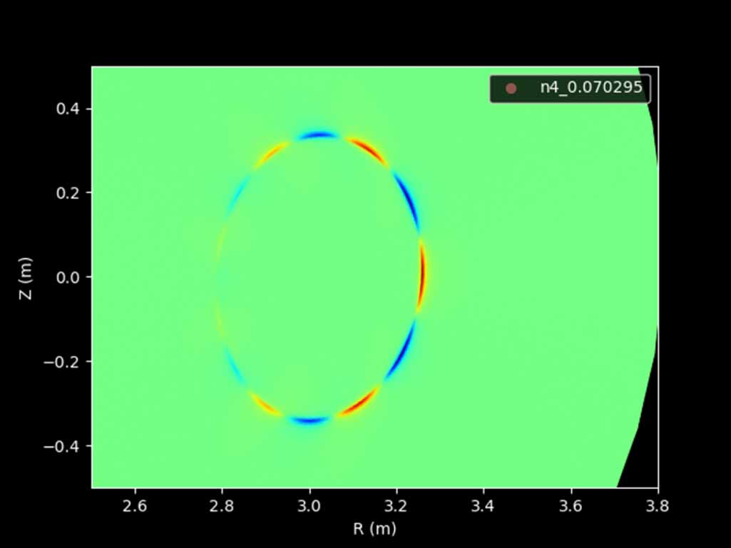
  . These are broad modes that couple a large number of poloidal harmonics and if unstable could transport fast ions a significant portion of the minor radius. Also presented are plots of the expected perturbed density
  for the incompressible modes through the relation
  where the electron density on each flux surface
  is obtained from a combination of Thomson scattering and LIDAR. Both modes produce density perturbations starting from
  on the outboard side extending to the edge at 3.8 m. This can be compared directly with the reflectometry data in figure 5. Although details of the amplitude as a function of radius are not available, evidence for the mode on reflectometry is only detected on the outboard towards the edge rather than in the core.
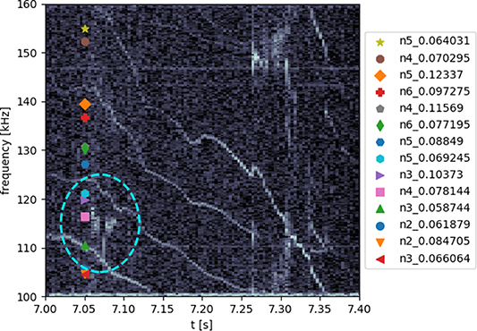
Figure 8. All MISHKA predictions of TAE frequencies overlaid on the spectrum obtained from interferometry in shot 99946. Modes have been labelled with a combination of toroidal mode number and eigenvalue. TAE signal circled.
Download figure:
Standard image High-resolution image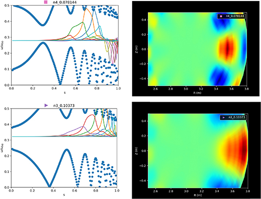
Figure 9. MISHKA predicted TAE eigenmodes which had frequencies the closest match to experiment. The n = 4 mode is presented top and n = 3 mode is presented bottom. Plotted left are the poloidal harmonics of  where
where  and
and  is the perturbed radial velocity, superimposed on the computed Alfvén continuum. Plotted right are 2D representations of the incompressible density perturbations
  .
.
Download figure:
Standard image High-resolution imageA detailed view of the mode frequency evolution is presented in figure 10. Rapid frequency chirping upwards on the millisecond timescale occurs early in the mode appearance. This does not appear correlated with ELM events and is not a broadband feature of the spectrum. ELMs can also be seen clearly on magnetics data in figure 4 at different times to the chirping. Given that it is unlikely that the bulk plasma equilibrium is changing on this timescale, a nonlinear wave process is a likely cause [34, 35]. This departure from linear physics is an additional ambiguity in identification of an appropriate linear mode since the frequency chirping of the mode is of order 5% which is of a comparable magnitude to the separation of predicted linear modes.
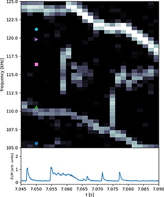
Figure 10. Zoomed spectrum obtained from soft x-ray measurements (top), and rescaled Be II photon flux from divertor (bottom) indicating timing of ELMs. Rapid variation of mode frequency appears uncorrelated with ELMs and is likely a nonlinear wave phenomenon. Linear MISHKA solutions presented in previous figures are also superimposed. Obtained from JET shot 99946.
Download figure:
Standard image High-resolution imageAlthough toroidal mode number is not available, the evolution of measured frequency with time provides further information on the frequency of the mode in the plasma frame. The plasma rotation falls during the afterglow, as can be observed with XCS data when CXRS is unavailable. It is straightforward to produce synthetic signals for how the mode at the position given by reflectometry should scale with time under the assumption that it has a fixed frequency in the plasma frame, and this is shown in figure 11, for direct comparison to figure 5. It is clear that as toroidal mode number increases, the effect of falling rotation should be more pronounced in the time evolution of a mode with large Doppler shift. We must conclude that the mode evolution is more consistent with a low toroidal mode number, and therefore, that most of the frequency in the lab frame consists of the plasma frame frequency. It is also informative to plot the TAE gap frequency evolution during the same time period, with the n = 3 gap plotted in figure 11. The TAE frequency rises during the afterglow because of the root inverse relationship to density for Alfvénic modes. This scaling with density is consistent with the time evolution observed in figure 5.
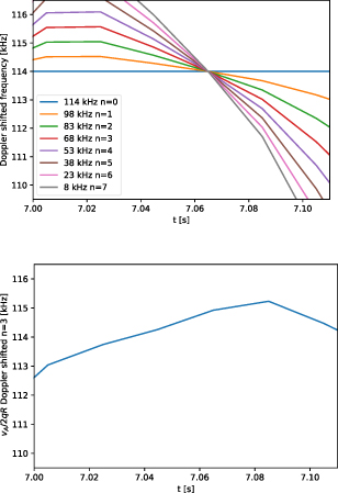
Figure 11. Synthetic spectra for a mode observed at 3.6 m under various assumptions. The top figure assumes a constant frequency in the plasma frame, but a Doppler shift that varies with time. The bottom figure tracks the n = 3 TAE gap frequency also including Doppler shift. These are scaled for comparison with figure 5. Both figures use XCS rotation data as an approximation to the rotation at 3.6 m.
Download figure:
Standard image High-resolution imageBefore considering drive and damping mechanisms, we summarize the evidence so-far for the signal being a TAE: the mode must be a magnetic perturbation because it is visible on Mirnov coils. The mode is measured by reflectometry to be located in a region of the plasma where the rotation would require a toroidal mode number of  for a zero plasma frame frequency. The nonlinear harmonics of low frequency activity in figure 8 show a clear trend downwards in frequency indicating how such a highly Doppler shifted non-Alfvénic mode should evolve during the brief observation, however the observed mode frequency is largely constant if not increasing. Therefore, although toroidal mode number is not measured, Doppler shift must not play a large role in its frequency, implying
  and a finite frequency in the plasma frame. The time evolution is consistent with Alfvénic scaling because the mode frequency rises with falling density. The mode lies within the band of frequencies predicted for TAEs using a restricted set of toroidal mode numbers chosen based on DD versions of the same discharges where RF driven TAEs were observed. Noting that previous TAE frequency predictions on JET with MISHKA obtain the mode frequency correct to a few percent [9, 36, 37], we have only selected TAE candidates within 5% of the observed modes. Both those candidates are consistent with a low toroidal mode number eigenmode producing a density perturbation on the outboard midplane with an absence of activity in the core. The modes that best match the observed frequency are much broader and further outside the core than modes driven by hydrogen minority in DD, consistent with drive by particles with a much larger orbit-width. This is also completely consistent with extrapolated predictions made in our previous work [9], although for earlier in the afterglow than considered before.
Having identified two likely candidate TAEs for alpha particle driven modes, we proceed to calculations of their linear drive and damping to examine if there is reason to believe that these particular modes should be the most likely to be observed of all the TAEs possible.
4.3. Fast ion linear stability
The appearance of TAEs on JET is typically attributed to a wave-particle resonant interaction with fast particles, where the basic mechanism of inverse Landau damping is well understood and in agreement with the fact that TAEs have never been seen in ohmic JET plasma. The linear drive and damping corrections to the MHD linear stability are valid provided the drive is weak, or equivalently, the motion of the resonant population is a small fraction of the wave energy. This linear drive from a given fast particle species depends on the equilibrium distribution function of that species, as expressed in equation (6). The sections below detail linear stability calculations for the alpha particles and NBI equilibrium distributions obtained at the time of interest 7.05 s
4.3.1. Alpha particle drive.
The alpha particle distribution function which is supposed to provide the drive is not measured in sufficient detail to provide input to stability analysis, although the presence of confined alpha particles is certainly measured in these plasmas (for example, using gamma ray emission) and will be discussed in other publications currently in preparation [38]. The alpha particle equilibrium distribution, neglecting any losses due to imperfect toroidal symmetry or mode activity, is expected to have the form of a slowing down distribution [39] similar to that used to represent NBI distributions, but for much larger energies and approximately uniform pitch angle distribution.
The assumed distribution function for alpha particles was taken to be
with  the field at the magnetic axis and
  the proton mass, where the alpha density profile prediction
  was taken from TRANSP [40, 41] and only the on-axis temperature was used to avoid the complication of a spatial dependence in the normalization factor
  . Two representations of the relationship between density in TRANSP and distribution function were considered: the finite orbit width (FOW) version and the zero orbit width (ZOW) version. Whilst it seems better to choose the
  option, the correction applied presupposes that the term (
 remains positive, which will not be the case for deeply trapped particles that are mirror reflected before
  . To make matters worse, these trapped and often non-standard orbits are exactly the orbits where these corrections would be the most important. It is difficult to argue that this FOW method is more consistent than the ZOW version, particularly considering how
  is already the result of a flux surface average of the function
  . Neither are faithful to the much more computationally challenging full Monte Carlo form, but both have the advantage of being smooth functions which will have well behaved gradients in 3D constants of motion space. Both representations were used as inputs to stability calculations to probe the sensitivity to these effects, which change both the value of the radial gradients
  and their location.
Full-orbit calculations of the wave-particle linear growth rate were computed with the perturbative code HALO [42] based on the FOW and ZOW versions of the alpha distribution function. These calculations assume that the eigenmodes computed with MISHKA are good representations of the electric and magnetic fields, and that the drive is sufficiently weak that the resonant fast alphas are not copious enough to change the mode structure.
The results of the linear HALO calculations are presented in figure 12. Both the calculations for ZOW and FOW give a positive growth rate for many of the TAEs, but certainly with some variation. Both calculations show the largest growth rates for  which is lower than what was found both theoretically and experimentally for minority hydrogen driven modes in DD, where the maximum was for
  Whilst it is true that the radial drive is directly proportional to
  in equation (6), the power transfer is sensitive to the orbit width and the Larmor radius. The work done by a particle drifting from one magnetic surface to another is maximized if the length scale of the drift matches the width of the mode which generally decreases with increasing toroidal mode number. This narrowing of mode width also means that it becomes comparable to the Larmor radius of the alpha particle, scaling similarly to the
  term seen in standard gyrokinetic and quasilinear equations, where
  is the Bessel function of the first kind and zero order. These findings should be compared again with modes overlaying the spectrum in figure 8. Concluding that any TAE driven by alphas should either be
  or
or  narrows the frequency window to between
  . However, we have been more stringent and matched the frequency and position of the modes to either
  or
or  078144 depicted in figure 9. For the ZOW distribution, these modes are within 10% of the highest growth rate, and for the FOW version, they are within 20%. This good correspondence between the most strongly driven modes calculated and the modes observed is also what occurred in DD for a completely different set of core localised modes driven by ICRH [9].
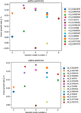
Figure 12. HALO full-orbit calculations of the linear drive of MISHKA TAEs. The results of the ZOW representation are given (top) as well as the FOW representation (bottom). Both calculations show that the n = 3 and n = 4 candidates have among the strongest drive of all the MISHKA modes.
Download figure:
Standard image High-resolution imageIt is important to understand how alpha particles generated in the core can be responsible for driving modes in the edge, and why the core modes are not the TAEs that are most strongly driven. Addressing the latter question is straightforward on inspection of a typical core mode in figure 13. Core localized modes in the low shear region have poloidal harmonics with much narrower radial scale lengths than those found in the finite shear region, and are a poor match for resonant alpha orbit widths (even being less than the Larmor radius of MeV range alpha particles). The power transfer density  between waves and particles scales linearly with the ratio of poloidal harmonic width
  to orbit width
  when
when  [43, 44].

Figure 13. 2D representation of the incompressible density perturbations  for a core localised TAE.
Download figure:
Standard image High-resolution imageTo answer how alpha particles generated in the core can be responsible for driving modes in the edge, we investigated the power transfer for the most promising n = 3 mode in figure 8. The HALO code was run with a fixed mode amplitude  for 30 wave periods, and the accumulated power transfer of ∼15 million alpha particle markers uniformly distributed in position and velocity
  phase space was recorded. A sample of the ∼500 000 most significant markers is presented in figure 14, along with two representative orbits for the resonances. The representation is given in invariant coordinates with
  . Red denotes damping contributions, whereas blue denotes drive.
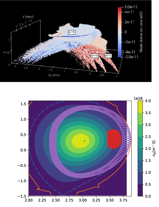
Figure 14. HALO full-orbit calculations of the wave-particle transfer between the n = 3 TAE and alpha particles. A selection of 500 000 markers with the highest power transfer sampled from 15 million markers are shown, with some resonances labelled (top). Also shown (bottom) are two typical 3 MeV orbits from the trapped and passing resonances superimposed on the contour plot of alpha density from TRANSP.
Download figure:
Standard image High-resolution imageThe four prominent red resonance surfaces in the figure correspond to  (cf equation (6)) and are caused by co-passing particles interacting with the TAE poloidal harmonics
  , increasing right-to-left in the figure towards the edge of the plasma. Despite being near the edge of the plasma where
  is large and positive, large contributions from
  in
in  push these branches into
  . The co-passing example orbit (purple) shows how fast alphas born on the inboard side in regions of appreciable fast alpha density gradient cross flux surfaces outwards and reach the outboard edge where the TAE is located. Similarly, resonances appear in blue for the deeply counter-passing particles
  .
.
An entirely different contribution comes from the trapped particle population with  . The blue band in the figure corresponds to the precessional resonance
  . A deeply trapped example orbit (shown red in figure 14 bottom) illustrates how alpha particles born towards the outboard edge of the ITB can travel across flux surfaces outwards to interact with the outboard TAE.
Having established that alpha particles can drive most of the TAEs identified, and how those in the edge with the frequencies closest to the experiment are some of the most likely to be observed, we examine how the drive compares with the predicted damping mechanisms.
4.3.2. NBI damping.
A significant motivation for the afterglow scenario was to remove the NBI and decrease the ion Landau damping from the fast NBI population. However, the time of appearance of the mode was only 50 ms after NBI turnoff. The decay time of neutrons exhibited in figure 2 demonstrate that an appreciable fast NBI population is present for at least 200 ms. The discrepancy warrants some calculation of the NBI contribution to damping during the time of interest.
The equilibrium distribution functions predicted for the 50:50 DT beams were computed via Fokker-Plank Monte Carlo simulation using the LOCUST code [45], based on beam source data computed with TRANSP. Markers are tracked in full-orbit until thermalization and then binned to produce the distribution  for input into HALO. LOCUST uses large numbers of markers to produce smooth distribution functions that give converged results for growth rates in HALO with minimal post-processing [46].
To allow rapid drift-kinetic calculations of NBI damping without including full-orbit physics for the sub 100 keV ions, a newly implemented guiding-centre orbit-following option in HALO has been implemented based on the Littlejohn Lagrangian formulation [47] allowing for order unity time varying electromagnetic fields [48]
taking  as a constant of the motion and
  as an ignorable coordinate. The guiding centre phase variables
  are integrated in time via a Runge-Kutta-Fehlberg 4th order scheme [49]. This functionality has been found to give the same results as the existing 'drift' mode available in HALO [42] but without having to track the entire gyration of the particles. This gives roughly a factor of 100 improvement in computation time in exchange for the loss of the long term phase space conserving qualities, which are of no consequence in linear calculations. It should be noted that these drift calculations of damping will be too high by a factor
  and therefore should be taken as either accurate or slightly pessimistic depending on the mode.
The results of the NBI damping calculations for the LOCUST distributions are given in figure 15. Modes with the lowest frequencies found in the central low shear region experienced the largest damping with  exceeding even the strongest alpha driven modes. This is as expected for a beam population that is largest in the core where these low frequency TAEs are found. Conversely, we see that for external modes, the damping is below
  . For the
  candidate TAEs of interest, the damping rates are
  and
and  respectively. For the
  mode, this still leaves
  of the alpha drive available.
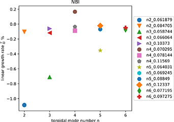
Figure 15. HALO drift calculations of NBI damping due to deuterons and tritons, using distributions computed with LOCUST.
Download figure:
Standard image High-resolution image4.4. Bulk nonideal linear stability
4.4.1. Ion Landau damping.
The resonant interaction between bulk thermal ions and the TAE modes have been previously calculated to be weak [9], however those calculations assumed the appearance of modes later in the afterglow at 100 ms rather than the 50 ms observed here. Linear drift-kinetic calculations of the ion Landau damping were therefore carried out using HALO in a similar manner to that performed for the NBI damping calculation. Two Maxwellian distribution functions were constructed using experimental values of ion temperature and density, assuming a 50:50 DT concentration. The plasma was taken to be in local thermal equilibrium with a flux surface spatial distribution of profiles  and
and  . The results of the ion Landau damping calculation are given in figure 16. The degree of ion Landau damping is generally small, with the exception of some core localised modes. In particular, the candidate n = 3 and n = 4 TAEs are found to damp at a rate comparable to their computed drive; the damping value of
  for the n = 3 mode is below the ZOW alpha drive calculation but above that found for FOW drive. The net drive of the n = 3 mode above ion Landau damping would therefore be at a rate comparable with the uncertainty in our method.
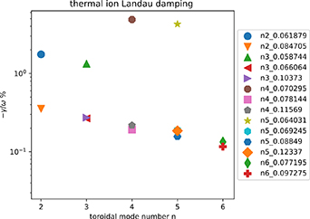
Figure 16. HALO drift calculations of ion Landau damping with D and T ions.
Download figure:
Standard image High-resolution image4.4.2. Radiative and collisional damping.
For all the MISHKA modes identified, equivalent modes were computed with the CASTOR code including complex resistivity (equation (5)). The complex resistivity value was computed at the location of each mode using experimental values for magnetic field, electron and ion temperatures and electron density. A code limitation meant that one value of the resistivity was given for the entire domain, however the resistive contributions are only expected to be appreciable at the location of each poloidal harmonic of the TAE mode where the field gradients are largest [13]. For narrow core-localised modes with low shear, this will be a well-defined location and a large effect, but for the broad edge localised modes, this is more ambiguous. As described in previous work [15, 50] and in our previous DD study, the radiative damping contribution for a mode is identified by re-calculating the MISHKA mode with CASTOR including the imaginary contribution to the resistivity computed from experimental profiles, and scanning the real part of the resistivity. The radiative damping rate is obtained by identifying the point at which the extrapolated plot of the mode damping rate intersects the zero-resistivity axis. The collisional damping is obtained by setting the imaginary resistivity to zero, and using the best available estimate for the plasma resistivity, in this case obtained from TRANSP calculations of neoclassical resistivity [51]. The results of both calculations are presented in figure 17.

Figure 17. The results from the CASTOR code. The radiative damping calculation for the TAEs computed with the imaginary resistivity (top) and collisional damping using real resistivity (bottom).
Download figure:
Standard image High-resolution imageThere is variation in radiative and collisional damping with mode frequency and mode number. Both have the effect of making the modes narrower in comparison with the non-ideal length-scales where finite parallel electric field and ion Larmor radius terms sensitive to field gradients begin to become important.
For the radiative damping, a very clear distinction can be made between the few narrow core localised TAEs which exhibit strong damping, and the majority of modes found in the finite shear region towards the edge of the plasma. The existence of core-localised TAEs is a finite aspect ratio effect which depends on the pressure gradient and local shear, with solutions at the bottom and the top of the TAE gap [52]. For a given pressure gradient, the frequency separation between the core TAE eigenfrequency and the continuum scales as  for inverse aspect ratio
  , radial derivative of Shafranov shift
  , and magnetic shear
  . As the pressure gradient increases, these core-localised modes decrease their distance to the Alfven continuum, becoming more narrow as they begin to more resemble singular eigenfunctions found in the continuum, with the upper modes entering the continuum first. For this equilibrium, no modes are found near the top of the TAE gap, however modes very close to the continuum are still found near the bottom. An example core localised TAE is presented in figure 18. This TAE is the same example given in figure 13 when discussing weak alpha particle wave-particle power transfer for narrow modes. It is therefore evident that two separate effects reduce the liklihood of observing core TAEs, and that modes near the edge, such as the candidate TAEs n3_0.10373 and n4_0.078144, are the most likely to be observed. It should be mentioned that when the radiative damping is so strong, the non-ideal bulk plasma effects on the core TAE mode structure will change the eigenmode, and indeed these changes were observed in the non-perturbative calculations in CASTOR. The improved CASTOR mode structures were not used in the alpha particle drive calculation, but are still very unlikely to put the drive of core (non-ideal) TAEs beyond the substantial damping.

Figure 18. 1D radial eigenfunction for a core localised TAE, super imposed on the Alfven continuum.
Download figure:
Standard image High-resolution image4.4.3. Total linear stability.
We summarize the results of the linear drive and damping calculations in figure 19. Given we have two different calculations of the alpha particle drive, we have used the difference in calculations as an attempt at quantifying the epistemic uncertainty. Propagating experimental uncertainties in the equilibrium, particularly the safety factor, is difficult because the MHD modes themselves will change in frequency, location, and spatial composition, if the equilibrium change is large. Assuming a perturbative analysis that keeps the mode structure fixed but varies  and the Alfvén speed in the approximate mode frequency
  , a ∼10% change in
  will be the dominant contribution. This change in
  will also change the orbit width
  . Both these effects are captured in the
  scaling in the wave-particle linear growth rate [5], changing both drive and damping equally by ∼20% for ion Landau damping, NBI and alpha contributions. Assuming that our eigenmodes are not too different to the true oscillations supported by the plasma, we then conclude that our dominant error in net drive is in the assumed form of the alpha distribution rather than the equilibrium.

Figure 19. Summary of contributions to linear growth rates for MISHKA TAE modes. The alpha drive given is the ZOW case, with the uncertainty estimated as the difference to the FOW case.
Download figure:
Standard image High-resolution image
A further complication is the variation in the fusion alpha source. The neutron rate measurement is found to vary by 8% around its peak value over the course of 30 ms. This is comparable with the short duration of the TAE observation. The nonlinear chirping of the TAE is known to extract energy from the fast distribution by flattening the radial gradients at resonance, which collisions then replenish, resulting in a cycle of chirps. The reduction of the alpha source on this timescale implies the replenished gradient will be lower and perhaps below threshold for instability. Whilst this may explain the short duration of a marginally unstable TAE, we can only speculate as these changes are within our uncertainties. It is perhaps also interesting to consider the timescale for alpha particles to slow down  to a given energy
  given by the Stix estimate
 ![$\tau = \frac{{{t_s}}}{3}\ln [ {1 + {{( {\frac{{3.52}}{{E\left[ {{\text{MeV}}} \right]}}} )}^{\frac{3}{2}}}} ]$](https://content.cld.iop.org/journals/0029-5515/63/11/112006/revision1/nfacee14ieqn177.gif) with
with  the Spitzer slowing down time [26]. Using this estimate, alpha particles slow to below 3 MeV at 32 ms, which will already depopulate some of the p = 0 precessional resonance in figure 14. After 54 ms, alpha particles are estimated to be below 1.7 MeV and no longer able to resonate with the precessional resonance. The loss of this alpha particle drive contribution is also a plausible reason for the brief duration of the unstable TAE.
It is clear from the results that the most important requirement in the appearance of alpha driven TAEs is the total absence of warm plasma physics, mainly through the radiative coupling to the kinetic Alfven wave. In the core where modes are narrower and the plasma is hotter, the finite ion Larmor radius and appreciable ion velocity from bulk ions both work to suppress TAEs well beyond what the alpha particles can overcome. We have found several TAEs for which these effects are not relevant. They are broad modes found near the edge of the plasma where the plasma is colder. These modes are neither strongly driven nor strongly damped, but lie dormant in the high magnetic shear edge region unless alpha particles generated in the core can become appreciable near the edge. For the calculations we have performed, we find that just before the time of experimental TAE observation, the ion thermal Landau damping and alpha particle drive for the candidate TAEs are equal within the error of our method. As the ion temperature decreases during the afterglow, we would of course expect the ion Landau contribution to continue to fall leaving a net alpha particle drive and a low amplitude TAE as has been observed.
5. Conclusions
The JET DT ITB afterglow scenario 99946 has been examined for TAE stability in light of a TAE mode observation. Many of the features of the observations support the stability calculations which identify it as an edge localised  or
or  mode in the incompressible linear ideal MHD spectrum, in line with other observations of TAEs at JET in the past. The appearance of this mode despite small alpha particle drive is possible because the radiative damping and NBI damping are also small, which is not true of modes predicted in the core. The mode appears early in the afterglow as the ion temperature drops and the bulk ion Landau damping decreases. Predictions of the alpha particle drive using different representations of the alpha particle distribution change whether this mode is predicted to be marginally stable or unstable. The appearance of the broad outboard TAE mode is partially a consequence of the large orbit-width of trapped alpha particles having precessional motion which matches the toroidal phase velocity of the TAE. This is a rather different wave-particle interaction mechanism than that expected for ITER [53] where the alpha particle orbit widths will be smaller and the conventional
  resonance will play a more important role in destabilization. This is also a curious finding in light of TFTR results [54] where core-localised modes were observed. Their detection limit for alpha driven modes was experimentally found to be for
  ,
,  and
and  , with clear modes observed for
  and
and  which are closer to our conditions. However, their results were achieved
  at higher field
  where non-ideal damping effects which scale as
  were smaller.
It is important to emphasise however that our stability analysis used on JET DT data is sufficiently general as to apply to ITER as well. Indeed, most complications in the linear theory come from studying large scale burning plasma but on smaller and less performant scales. Elaborate effects such as FLR, finite orbit width, and the precession of non-standard orbits have been required to understand our existing data on top of the same fundamental physics that governs TAEs on ITER. Moreover, being far from burning plasma at Q<1.0, our stability methods have required higher accuracy to successfully predict weakly alpha driven modes. Accurately predicting the stability of a TAE with linear drive  is a much more difficult proposition than the
  drive expected in the ITER baseline [55] but can use the same tools.
These results reinforce the finding that the bulk thermal plasma is responsible for suppressing the TAE instability in the presence of alpha particle populations, and improvements to the modelling of non-ideal effects such as radiative damping and Landau damping are required for quantitative predictions when these alpha effects are still weak.
Acknowledgments
This work has been carried out within the framework of the EUROfusion Consortium, funded by the European Union via the Euratom Research and Training Programme (Grant Agreement No 101052200—EUROfusion) and from the RCUK Energy Programme (Grant Number EP/P012450/1). Views and opinions expressed are however those of the author(s) only and do not necessarily reflect those of the European Union or the European Commission. Neither the European Union nor the European Commission can be held responsible for them. To obtain further information on the data and models underlying this paper please contact PublicationsManager@ukaea.uk.