


Abstract
Safety factor profile control via active feedback control of electron temperature profile during a plasma current ramp-up phase of a DEMO reactor is investigated to minimize the magnetic flux consumption of a central solenoid (CS) for wide range of q profiles. It is shown that q profiles with positive, weak and reversed magnetic shear can be obtained with the resistive flux consumption less than 60% of the empirical estimation which is calculated using the Ejima constant of 0.45. For the optimization of the target electron temperature profile and feedback gain to control electron heating power, reinforcement learning technique is introduced. One important feature of the system trained by reinforcement learning is that it can optimize the target electron temperature adaptive to the present status of a plasma. This adaptive feature of the reinforcement learning enables to control q profiles even in the case that an effective charge profile is randomly modified and it is not measured directly.
Export citation and abstract BibTeX RIS
1. Introduction
Safety factor profile shape is one of major ingredients to define tokamak operation regimes because confinement and stability of a tokamak plasma is closely related to it, therefore it is indispensable to tailor a q profile in a current ramp-up phase for a tokamak reactor. Historically, it was shown in many tokamak devices that q profile control can be done by auxiliary heating during current ramp-up phase [1–4]. On the other hand, it is also widely known that the poloidal flux consumption of a central solenoid (CS) can be reduced by the auxiliary heating during the current ramp-up phase [5–7]. If a CS flux consumption in current ramp-up phase is reduced, a tokamak reactor design with a smaller CS might be possible. Since the design margin of a DEMO reactor is very small, it is important to quantify the minimum value of required CS flux. Basically, as the heating power increases the amount of reduction of a flux consumption increases and at the same time a q profile tends to be changed from a positive shear (PS) profile to a weak shear (WS) or a reversed shear (RS) profiles because the diffusion of the plasma current slows down. This constraint might restrict q profiles, and consequently operation regimes in DEMO reactor if a large reduction of a CS flux consumption is required. However, if an electron temperature profile which is sufficiently peaked can be obtained by on-axis electron heating, this constraint is thought to become loose because the reduced resistivity at the core region has an effect to increase the plasma current in the core and counteracts the slow down effect of the current diffusion.
Based on this idea, we have shown the existence of the optimum electron temperature profiles which provides the minimum CS flux consumption under a given time evolution of q profile in our previous study [8]. Note that, the effect of current drive on the reduction of resistive flux consumption in current ramp-up phase is small as discussed in our previous study, therefore the effect of electron heating, instead of direct current drive, is treated in this paper. The flux consumption of external coils including CS can be divided into three components. The first two components are an external and an internal inductive flux consumption ( and
and  ), which are converted to the poloidal magnetic flux produced by the plasma current outside and inside the plasma surface. The third component is a resistive flux consumption
  , which corresponds to the resistive dissipation of the magnetic energy [9]. The sum of
  and
and  cannot be reduced if we fix a plasma shape and a q profile at the end of current ramp-up. On the other hand, it was shown that a large reduction of
  is possible by the optimization of electron temperature profiles.
However, it was not shown that the optimum electron temperature profiles proposed in our previous study can be realized by the electron heating at finite locations. In this study, we try to obtain these electron temperature profiles by the feedback control using near axis and off axis electron heating. In order to control an electron temperature profile appropriately, we need to optimize a feedback control gain considering the transport property of the plasma. This is the first optimization problem dealt with in this paper.
A major drawback of our previous study is that the optimum temperature profiles proposed was calculated assuming a predetermined flat effective charge  profile. In order to overcome this restriction, we also investigate the way to optimize the target electron temperature profile according to a
  profile. However, it is usually difficult to measure a
  profile in real-time manner, therefore we need to find an optimum electron temperature profile without a direct measurement of a
  profile. This is the second optimization problem dealt with in this paper.
For both optimization problems treated in this paper, we estimate that a main difficulty comes from that the solution should be modified adaptive to the active response of plasmas. In order to overcome this difficulty, we introduce reinforcement learning technique. The reinforcement learning technique will be able to construct adaptive control systems through trial-and-error.
This article is organized as follows. Outline of reinforcement learning technique is explained in section 2. The results of q profile control with reduced resistive flux consumption are shown in section 3. Firstly, an optimization of feedback control gain for  profile control with electron heating power is explained in section 3.1. Secondly, the results of q profile control for wide range of target q profiles are shown in section 3.2. In this subsection, the target electron temperature is calculated using the way shown in our previous study. In section 3.3, we introduce the second reinforcement learning system to optimize target electron temperature profile for randomly selected
  profiles. In the last subsection of section 3, the possibility of q profile control with reduced resistive flux consumption using electron heating for a plasma with randomly selected
  profile is shown, and conclusions are given in section 4.
2. Reinforcement learning technique
Reinforcement learning is one of a class of machine learning. The aim of reinforcement learning is to find a solution to a problem such as a control problem through trial-and-error. A learning process called as an agent tries to find a solution of a problem through interaction with an environment (e.g. plasma). The agent interacts with the environment through actions (e.g. control of heating power). The environment is affected by the actions at the previous time step. As a measure of goodness of each action, a reward value is defined based on the state of the environment. For example, a high reward value is given if the control residual of electron temperature profile is small. The agent tries to maximize the sum of rewards obtained through a chain of actions. One of an important feature of the reinforcement learning is that it can adaptively optimize actions using the input signals describing the state (e.g. the electron temperature profile) of the environment. For example, we expect that the system obtained by reinforcement learning can optimize the heating power for control of the electron temperature profile adapting the thermal transport and confinement property of the plasma.
A detailed description of algorithms of reinforcement learning can be found on an introductory book [10]. We here describe an outline of the learning procedure of the actor-critic algorithm which is a type of reinforcement learning algorithms we use. The framework of the actor-critic algorithm is summarized in figure 1. The actor-critic algorithm consists of a policy function  ('the actor') and an action-value function
  ('the critic') where a state s denotes parameters describing an environment and a is a set of actions. The policy function determines what actions to take at the state s and the action-value function estimates a sum of rewards which will be obtained when an action a is taken at a state s and succeeding actions are chosen based on a policy
  . The action-value is defined as
where rt is a reward at time step t and  denotes the expectation based on a policy function
  . Note that a policy function can be probabilistic. Both the policy function
  and the action-value function
  are approximated using neural networks whose weight parameters are defined as
  and
and  . The approximated action-value function
  is trained to reduce the difference between the actual sum of rewards obtained in each trial and the estimation based on
  . To train the policy function
  , a gradient of an estimated sum of rewards with respect to
  is calculated using
  [11]. By updating weight parameters of a policy function
  using this gradient, we expect that a sum of rewards increases when actions are taken based on a new
  .
.
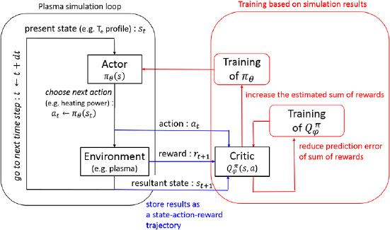
Figure 1. Flamework of the actor-critic argorithm. Black arrows represent a time step of the trial. Blue arrows represent the storage of results as a state-action-reward trajectory. Red arrows represent the training of the policy function  and the action-value function
  . The training process takes place after a certain length of state-action-reward trajectory is completed.
Download figure:
Standard image High-resolution imageCompared with the problems commonly treated in the benchmark of reinforcement learning algorithms such as video games and control simulations of robotic systems, it takes much longer time for an integrated transport simulation of the plasma. Therefore, we need to choose an algorithm which can learn with parallelized multiple agents to increase a number of trials per unit time and can learn from relatively small number of trial data. Amongst state-of-the-art reinforcement learning algorithms, ACER [12] fulfills this requirement because it is learnable with multiple agents and it has a functionality called experience replay [13]. Experience replay is technique to reuse previous results of trials for the present leaning, which improves the efficiency of leaning. We use an ACER implementation on Chainer [14], an open source framework for deep learning.
3. Safety factor control with reduced resistive flux consumption utilizing reinforcement learning
In this work we perform the time dependent transport simulation for the DEMO reactor using TOPICS [15] integrated modelling code suites. We use CDBM model [16] as a turbulent thermal transport model and a prescribed density profile is used. As for parallel electric resistivity, we use a neoclassical resistivity [17]. Physical parameters such as plasma size, required plasma current at the flat top and locations of external coils are taken from the steady-state DEMO reactor design JA Model 2014 [18]. The fusion output of this reactor is 1.5 GW, the major radius R0 is 8.5 m, the minor radius a0 is 2.6 m, the elongation is 1.65, the toroidal magnetic field is 5.9 T, the plasma current  is 12.3 MA at the flat top, the safety factor at 95% of the magnetic flux surface q95 is 4.0. Since an initial plasma is thought to be diverted around the plasma current of 3.3 MA and a substantial auxiliary heating power can be applied after this phase, the plasma current ramp-up phase from 3.3 MA to 12.3 MA is investigated in this study. Plasma shape is almost fixed because the currents of external coils are calculated so that the plasma surface passes through 12 fixed control points throughout the ramp-up phase. The line averaged electron density is kept at 60% of the Greenwald density limit during the current ramp-up (see figure 4(a)). The resistive flux consumption during this phase can be estimated from an empirical scaling law using the Ejima coefficient (
 –0.5) as
  [19]. If we assume that
  ,
,  to reach
  and 12.3 MA can be calculated as 16 Wb and 59 Wb, respectively, thus the resistive flux consumption during the current ramp-up phase can be estimated as 43 Wb. We here assume the same
  is applicable to the plasma start-up phase before reaching
  and the succeeding current ramp-up phase. This assumption is based on the experimental results on JT-60U [20] and DIII-D [21].
3.1. Optimization of feedback control gain
To control the electron temperature profile, we here assume that electron heating is applied at  and 0.6. Since the electron heating at one location may affect not only the electron temperature at the heated location but also the other controlled locations, an integral gain matrix with off-diagonal terms are used. The state at time t is defined as
where  and 0.6,
  is the electron heating power,
  is the electron temperature,
  is the target electron temperature and e is a control residual of
  defined as
  . The action a consists of
  terms of feedback gain matrix. These four gain terms are decided based on the output of the policy function
  . The reward is defined as
where C is a normalizing constant of control residuals. The agent measures the state st every 100 ms and determines the gain matrix at this time step, then, electron heating power is updated using integral controller and proceed to next time step of transport simulation. This time step is long enough for  at
at  and 0.6 to respond to a change of the heating power and achieve a quasi steady state profile. Therefore, integral controller is sufficient to control
  profile because integral control is applicable for a reduction of a steady state error. We avoid to use proportional gain to reduce a number of gain terms to be optimized. In addition, this time step is short enough to control a safety factor profile because current diffusion time is roughly one or two order longer than this time step. Training of neural networks which approximate policy function and action-value function is performed when one case of plasma current ramp-up simulation is finished. The training is performed based on the information of state-action-reward trajectories of the present simulation and previous simulations. A result of optimization is shown in figure 2. In this case, a plasma current ramp-up from 3.3 MA to 4.1 MA, which is the first 5 s of plasma current ramp-up phase, is simulated. Control target of
  profile is taken from the optimum
  profile obtained in our previous study [8]. As shown in figure 2(a), the average error of the electron temperature is decreased as the simulation experience accumulated. After the 1050 times of simulations, the electron temperatures at
  and 0.6 follow the targets with properly controlled electron heating power as shown in figures 2(b) and (c). Learned feedback gain is shown in figure 2(d). It is clearly shown that the feedback gain to control
  at
at  by the electron heating power at
  (
( 22) is set high and off-diagonal terms (
 12 and
  21) are kept small. This result is reasonable because the effect of electron heating at different location has far small effect compared with that at the same location in our transport simulation.
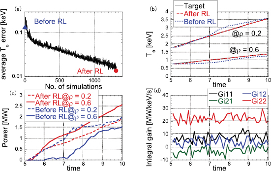
Figure 2. Results of feedback gain learning. (a) Time averaged  error at each ramp-up simulation. Blue triangle and red circle represent the simulations shown as results before and after reinforcement learning (RL) in ((b) and (c)). ((b) and (c)) Time evolution of
  and electron heating power at
  and 0.6. Black curves represent the target, red curves represent the result after the learning and blue curves represent the result before the learning. (d) Time evolution of integral gain terms in the simulation after the learning.
Download figure:
Standard image High-resolution imageThe progress of the learning can be confirmed by figure 3, the plot of the state-action function at the initial state  and a histogram of number of trials for each diagonal gain term are shown. At the beginning of the learning, no action is expected to give a high reward and the policy function is initialized to choose gains based on a normal distribution whose peak is near 0. As the number of trial increases,
  is trained to have a high value at a high gain for
  (
( 22) and a moderate gain for
  (
( 11) and at the same time, policy function is modified to have peak around that value (the x symbols in figure 3. denote the peak of policy function at each learning step). The peak of the policy function is located near the peak of the action-value function but they do not coincide. This is because the policy function is not updated to have a peak at the peak of the action-value function, instead, it is updated to increase a probability at the peak of the action-value at every leaning step and its change is kept rather small to avoid the instability during the learning. This is a feature of an actor-critic algorithm.
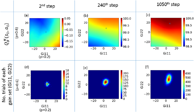
Figure 3. 2d contour of ((a)–(c)) action-value function at the first time step  and ((d)–(f )) histogram of number of trials of each gain set (Gi11, Gi22). Figures ((a) and (d)) shows the results at the 2nd learning step, ((b) and (e)) at the 240th learning step and ((c) and (f )) at the 1050th learning step. Blue x symbols in ((d)–(f )) denote the peak of policy function.
Download figure:
Standard image High-resolution imageFrom this result, it is shown that a feedback gain for the electron temperature profile control can be optimized using reinforcement learning technique. However, it is also estimated that once a fixed feedback gain is properly chosen, online adaptive optimization of feedback gain is not required for the electron temperature profile control in our transport simulation.
3.2. Safety factor profile control through electron temperature profile control using optimized feedback control gain
We have shown that  profile can be controlled by electron heating when its power is controlled by integral feedback controller whose gain matrix is optimized using reinforcement learning technique. Since we have already investigated the method to calculate the optimum
  profiles required to minimize the resistive flux consumption for arbitrary q profiles in our previous study [8], q profile control with minimized resistive flux consumption will be realized if these optimum
  profiles are realized using the feedback controller optimized as explained in the previous section. As we mentioned in the introduction, we want to obtain wide range of safety factor profiles from a positive shear (PS) profile to a weak shear (WS) profile and a reversed shear (RS) profile, therefore, we firstly prepare three types of target q profiles. We here imitate a simple experimental modification of a safety factor profile. A fixed heating power is applied at
  = 0.6 and it is changed shot by shot. As a result, we obtain three target q profiles shown as broken curves in figure 4(b) when 0, 2.5 and 7.5 MW of heating power is applied. Note that, feedback control of
  profile is not performed, and hence the resistive flux consumption is not minimized at this stage. We take these scenarios as reference scenarios before the minimization of resistive flux consumption, which are shown as open symbols in figure 4(c). We then calculate the optimum
  profiles for these target q profiles to minimize the resistive flux consumption. We perform
  profile feedback control simulations using these optimum
  profiles as target
  profiles.
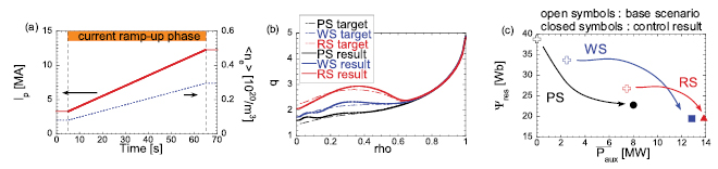
Figure 4. Results of the electron temperature profile control for the reduction of resistive components of CS flux in plasmas with q profiles with positive shear (PS), weak shear (WS) and reversed shear (RS). (a) Time evolution of the plasma current and the volume averaged electron density. The current ramp-up phase in which the electron temperature profile control is performed is highlighted. (b) Target and resultant q profiles at the end of the current ramp-up phase (65 s). (c) Resistive flux consumption and time averaged auxiliary heating power ( ).
).
Download figure:
Standard image High-resolution imageThe results are shown as solid curves in figure 4(b). The electron temperatures at two point are controlled with the electron heating at  and 0.6 and the q profiles similar to the target profiles can be realized. Note that the location of core heating is changed from
  to
to  to minimize the error of q profile especially in the core region,
  Resistive flux consumptions are reduced for three target q profiles as shown in figure 4(c). Since external heating power is not applied for a PS base scenario, the resistive flux consumption for this scenario is comparable to the previously calculated empirical estimation (43 Wb). There is a small discrepancy but it is within the margin of Ejima constant (
 –0.5). It is shown that the resistive flux consumption can be reduced less than 60% of the empirical estimation for a PS plasma and more reduction can be attained for a WS and a RS plasmas.
3.3. Optimization of target electron temperature profile
The target electron temperature profile for the q profile control in the previous section is calculated assuming the flat effective charge profile of 1.84 (which is the design value of JA Model 2014). To use this system in a real experiment, however, this assumption is rather strong since it is probable that  is not kept in a design value and it is also probable that
  is not spatially constant. In addition, it is difficult to measure
  profile in real-time manner especially in a DEMO reactor. Therefore, we shall not rely on the target electron temperature profile prepared in advance, instead, we should modify the target electron temperature profile which adapts to
  profile at the experiment without the direct measurement of it. For this purpose, another reinforcement learning is performed. Note that, although the method shown in this section is applicable for plasmas with wide range of q profiles including WS and RS profiles, the result for a PS plasma is shown in detail as a representative example.
In this section, we train a system which estimates an optimum target electron temperature profile from the information of state,
where  is a q profile at the time t,
  is an electron temperature profile at the time t,
  is loop voltage on a magnetic axis at the time t,
  is a target q profile at the next time step,
  is target loop voltage at the next time step and
  is the time at the end of current ramp-up. As is discussed in detail in our previous study [8],
  derivative of loop voltage can be inferred from time derivative of q. In other words, if time evolution of q profile is measured, loop voltage profile shape can be estimated but uncertainty of arbitrary offset remains. Therefore an additional information of this offset is given as loop voltage on a magnetic axis to estimate the absolute loop voltage profile. For the same reason, the target of q profile and on-axis loop voltage are included in the state st to control the q profile and the resistive flux consumption at the same time. In addition, the agent is given enough information to infer the relation between
  profile and loop voltage profile, or a parallel resistivity profile at each time step, which is dependent on
  . Therefore, it is expected that a well trained agent will be able to optimize the target electron temperature profile adaptive to the difference in
  . For example, a plasma with higher
  shows a larger difference between
  and
and  for the given
  and
and  , therefore, the agent can determine that a higher electron temperature will be required to obtain
  compared with a plasma with lower
  . Note that this system does not require a measurement of
  . Since we need target electron temperature profiles which can be realized by the control of electron heating at near axis and off axis locations and we expect a plasma which has no internal transport barrier, we restrict the target electron temperature profile as a combination of a flat profile at the on axis region (
 ), an exponential profile at the core region (
 ) and a linear profile at the peripheral region (
 ). As for
  profiles, we set
  , where Z0 and Z1 are the effective charge at
  = 0, 1 and cZ is a profile coefficient which determines the peakedness of a
  profile. Z0 and Z1 are randomly chosen between 1.5 and 3.5 but the difference between Z0 and Z1 is restricted less than 1 and cZ is also randomly chosen between 0.5 and 2.0. We assume that the
  profile is constant during the discharge. A reward is defined as
  , where rq is a reward concerning an error of a q profile and
  is a reward concerning an error of loop voltage, and therefore the resistive flux consumption. They are defined as
where Cq and  are normalizing constants of each error. Moreover, an additional reward
  is given at the end of current ramp-up to ensure that a q profile control residual at this point is minimized. The effect of this additional reward is discussed later in this subsection.
After several thousands of learning steps, the leaning agent becomes able to output an appropriate target electron temperature adapting a wide range of  profiles. As shown in figure 5, the q profiles are controlled with electron temperature profiles adaptively optimized for different
  values by the learned agent. It is clearly shown that the higher electron temperature is outputted for the plasma with higher
  , and as a result, the q profiles are controlled to almost the same profile. Although the results with flat
  profiles are shown in figure 5 as representative results, the same level of control is possible for the plasmas with non-uniform
  profiles. If the target electron temperature profile prepared in advance assuming
  is used, the resistive flux consumption increased as
  increases and the error of the q profile becomes large when
  as shown in figures 6(a) and (b). This issue is resolved by using adaptively optimized target electron temperature profiles. Although the solution seems to be trivial that increase in a resistivity due to increased
  is compensated by the increased electron temperature, the most important point is that this optimization is performed without the measurement of
  profile. This fact supports the conjecture that the information given as state s is enough to estimate the response characteristics of a q profile and loop voltage to the electron temperature, which depend on
  profile.
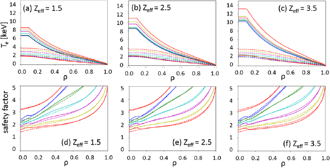
Figure 5. ((a)–(c)) Optimized target electron temperature profiles and ((d)–(f )) resultant q profiles at 5 s (red), 15 s (blue), 25 s (green), 35 s (cyan), 45 s (magenta), 55 s (yellow) and 65 s (red). The effective charges are 1.5 ((a) and (d)), 2.5 ((b) and (e)) and 3.5 ((c) and (f )). Dashed curves in each figure are the electron temperature profiles or q profiles of the base scenario in which no auxiliary heating is applied.
Download figure:
Standard image High-resolution image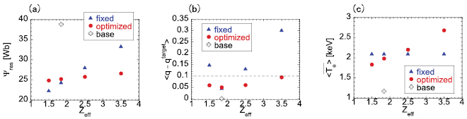
Figure 6. Comparison of results of (a) resistive flux consumption, (b) averaged error of q profiles at the end of the current ramp-up and (c) the time average of the volume averaged electron temperature. Blue triangles are the results when prescribed electron temperature profiles optimized for the plasma with  are used. Red circles are the results when electron temperature profiles are adaptively optimized by the learned agent. Black crosses represent the result of the base scenario in which no auxiliary heating is applied, which is the same result as shown in figure 4(c).
Download figure:
Standard image High-resolution imageThe effect of the additional reward at the end of current ramp-up can be understood with examples of control simulations when Z0 = 2.5, Z1 = 1.5 and cZ = 1.5, which is shown in figure 7. The agent learned without the additional reward cannot reduce the error of the q profile at the end of the current ramp-up less than 0.1, while the agent given the additional reward can reduce that as low as 0.06 but the loop voltage is slightly higher than the target. It is clearly shown that the agent is encouraged to minimize the error of a q profile especially at the end of the current ramp-up at the cost of increased errors of loop voltages with this additional reward. As shown in this example, a careful design of the reward is essential to control the performance of the agent in the reinforcement learning.
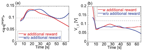
Figure 7. Comparison of results of (a) averaged error of q profiles and (b) error of loop voltage at magnetic axis. Red and blue curves show the control results using the system trained with or without an additional reward at the end of current ramp-up, respectively. Black solid curve in (b) represents  . Black dashed curves in both figures represents the error same as the normalizing constants, therefore the rewards rq and
  become
  on these curves.
Download figure:
Standard image High-resolution imageThe same level of q profile control and  reduction are also possible for a weak shear target q profile and a reversed shear target q profile. Although the error of q profiles becomes slightly higher for some
  profiles, they can be kept less than 0.18. The resistive flux consumption is reduced to the same level shown in figure 4(c).
The results shown in this section shows that the system trained for various  profiles can realize adaptive control. This fact shows that the assumption on a plasma parameter to design the control system can be reduced by using this system. This will apply to other important plasma parameters, such as the density profile. Therefore, this system has a potential to realize adaptive control which relies on less assumptions and it will be applicable for wide range of plasma parameters.
Note that we ignore the effect of measurement error in this paper. Real-time measurement of q profile are already realized in many tokamaks [22–25], however, it is generally difficult to measure time derivative of q profile with accuracy required to estimate loop voltage profile in the existence of the measurement error. The effect of the random error will be reduced by increasing the time step for the control and averaging a large number of observations. Since time evolution of q profile in a reactor condition is very slow, the same level of q profile control will be possible if the time step is substantially increased. On the other hand, the systematic error will be difficult to reduce. The sensitivity analysis of this system to the systematic error is remained as an important future work.
3.4. Realization of adaptively optimized target electron temperature by feedback control of electron heating power
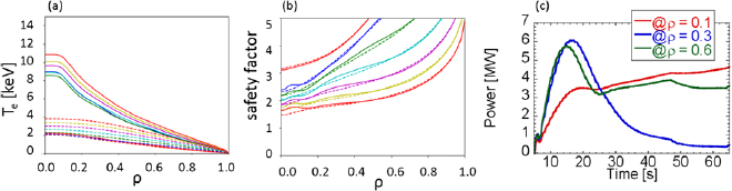
For the results shown in figures 5 and 6, the time evolution of the q profile is calculated for the exact target electron temperature profile determined by the system explained in section 3.3, that is, the temperature profile is not calculated based on the thermal transport equation. We have already shown that the optimization of a feedback gain to control the electron temperature profile by the electron heating power can be done by the system explained in section 3.1, we here check that the adaptively optimized target electron temperature profiles can be realized by the feedback control of electron heating at several locations. It is found that the target electron temperature profiles are well reproduced when electron heating power is applied at three locations where  , 0.3 and 0.6. As a result, the q profile control and a reduction of resistive flux consumption to the same level as the results shown in figures 5 and 6 is achieved as shown in figure 8.
Figure 8. Results when q profile control is performed using electron heating at  , 0.3 and 0.6. (a) Electron temperature profiles and (b) resultant q profiles at 5s (red), 15 s (blue), 25 s (green), 35 s (cyan), 45 s (magenta), 55 s (yellow) and 65 s (red). (c) Time evolution of electron heating power at
  (red), 0.3 (blue) and 0.6 (green). The effective charge is 2.5 in this calculation. The resistive flux consumption
  is 24 Wb, which is the same level of the optimized results shown in figure 6.
Download figure:
Standard image High-resolution image
It might be possible to learn the gain matrix to control q profile and  directly, however, the response of q profile to the heating power is far more complex compared with the
  profile and it is not clear that a simple feedback system like an integral controller is suitable for direct control of q profile. On the other hand, we have shown here that by combining two rather simple systems, q profile and
  control can be achieved.
4. Conclusions
The way to control a q profile in the current ramp-up phase with reduced resistive flux consumption is investigated. In order to control a q profile during the current ramp-up phase using electron heating at several locations, the target electron temperature profile should be optimized according to the  profile and the feedback gain to control electron temperature by electron heating should also be optimized. It is shown that reinforcement learning technique can be used to find a solution to these optimization problems. Using this technique, a reduction of resistive flux consumptions more than 40% is achieved for PS, WS and RS plasmas with a variety of
  profiles. One important feature of a system trained by reinforcement learning is its ability of adaptive optimization. This feature is clearly shown in the results of optimization of a target electron temperature profile for a randomly chosen
  profile. Input parameters are the present and previous status of the controller and the controlled object. These are enough information for the agent to infer a present response characteristics between the controller and the controlled object. The agent are thought to be able to optimize the action of the controller at the next time step based on this response characteristics.
Acknowledgments
The authors with to thank the developers of Chainer and its RL library ChainerRL because the large part of the programs used in this work take advantage of the algorithms implemented in their frameworks.