


Abstract
Collisional particle transport is examined in several toroidal plasma devices in the presence of perturbations typical of modes leading up to a disruption, of saturated tearing modes, or of unstable Alfvén modes. The existence of subdiffusive transport for electrons is found to occur in some cases at very low mode amplitudes and to also exist even for ions of high energy. Orbit resonances can produce long time correlations and traps for particle trajectories at perturbation amplitudes much too small for the orbits to be represented as uniformly chaotic. The existence and nature of subdiffusive transport is found to depend on the nature of the mode spectrum and frequency as well as the mode amplitudes.
Export citation and abstract BibTeX RIS
1. Introduction
It is well known that transport is not always diffusive in situations involving stochastic magnetic fields [1–4]. These publications evaluate the transport in terms of characterizations of the field, such as correlation lengths and times, related to the Kubo number, and the Kolmogorov length, and particle orbit properties such as the gyro radius and collision rates. But it is not clear from these publications to what degree the modification of particle diffusion will occur in typical plasma discharges. Of particular interest is the nature of ion and electron transport in the early stages of the onset of a tokamak disruption, or in the presence of small amplitude Alfvén modes, where the orbits are not uniformly chaotic and not simply characterized in terms of parameters assuming a homogeneous stochasticity. In the vicinity of stochastic threshold [5–8] there exist long time correlations due to remnant resonance islands that make the use of the random phase approximation [9] invalid to evaluate particle transport, and both simulations [10] and experiments [11] have indicated that its use can lead to incorrect results. Resonances produce long time traps that make the resulting particle distribution in time very nonuniform in space [7], and change the nature of the transport. In fact, at low amplitudes, when a magnetic surface breaks it forms a 'cantorus' (Cantor set) with gaps, which are the only places through which the field lines can escape. In the vicinity of one cantorus is an infinite Markov tree of cantori which slow the escape of particles, and cause them to linger or stick in that region for many toroidal turns, leading to subdiffusive transport [12]. We recall here that, given an observable of particle transport, which can be the toroidal canonical momentum  , we have subdiffusion when
  with
with  , ordinary diffusion when
  , superdiffusion when
  ,
,  being the time.
In the reversed field pinch in Padova, (RFX) [13, 14], where the amplitudes, phases, and structure of the saturated tearing modes are well known, the transport can be evaluated and is found to be subdiffusive [8]. It is clear that fitting subdiffusion with a diffusive scheme overestimates the rate of change of particle positions, especially if one focuses on the value of  , alone: often a too large value of
  must be compensated with ad-hoc terms, such as the 'pinch' or up-hill velocity [8], with unclear and often misleading results, especially if one extrapolates confinement with a diffusive scheme, as a function of perturbation amplitudes. In a preceding work [15] we have explored the connection between subdiffusion and nonlocality, showing that long-range correlations in particle motion (arising from particle trapping in sticky regions) make the diffusive assumption of a random, gaussian distribution of jumps invalid. On the contrary, a nonlocal model such as the Montroll master equation [16] captures the density evolution in the RFX device correctly. Alternatively, Zaslavsky [17] and others [18] used a transport equation with fractional derivatives by means of the factorization of the Montroll propagator into spatial and time functions. Both approaches (fractional and master equations) overcome the limits of the diffusive-convective scheme in describing subdiffusive systems. Nevertheless, the fractional derivative approach has the disadvantage of assuming an infinite homogeneous system and violating causality, it involves action at a distance in a zero time interval. The Montroll equation has neither of these defects.
In tokamaks the state leading up to a disruption is characterized by the presence of large scale tearing modes, often comprising modes with  , and
, and  , where
  and
and  are poloidal and toroidal mode numbers [19]. However, the initial state, with relatively small amplitudes, is very far from being uniformly stochastic, and standard methods of calculating transport by approximations which assume such homogeneity are not warranted. Furthermore, models which include particle trapping and the decorrelation of the trapping make assumptions about the nature of the traps and the process of release.
In this work we examine collisional particle transport in the presence of magnetic perturbations associated with instabilities commonly found in toroidal confinement devices. The nature of the particle transport is studied as a function of the magnitude of the perturbations, the particle energy, and the collision rate, to discover the onset of anomalous transport and its persistence for perturbation amplitudes above stochastic threshold. We use the cases of the slowly evolving large scale perturbations associated with the onset of a tokamak disruption, the saturated tearing modes seen in a reversed field pinch, and the high frequency short scale perturbations given by unstable Alfvén modes.
Particles are followed using the guiding center code Orbit [20]. The guiding center Hamiltonian is

where  is the normalized parallel velocity,
  is the magnetic moment, and
  the electric potential. The field magnitude
  and the potential may be functions of the poloidal flux
  , the poloidal angle
  and also the toroidal angle
  if axisymmetry is broken.
The equations of motion in Hamiltonian form are
where canonical momenta are

and  is the toroidal flux, with
  , the field line helicity. The functions
  and
and  pertain to the equilibrium, with
  giving the toroidal and
  the poloidal field magnitudes.
The equations of motion are easily generalized [21] to include flute-like perturbations of the form  with
with  the equilibrium field and
  . The perturbation
  has units of a length, simply related to the cross field ideal displacement produced by the mode, and is normalized with respect to the major radius of the device. We consider modes with frequency much smaller than the cyclotron frequency, so the magnetic moment
  is conserved. Tearing modes have long scale lengths, so the averaging produced by gyro motion is not expected to be significant, but to be certain to include any such effect for Alfvén modes with short scale lengths, we have included four point gyro orbit averaging in the guiding center analysis of high energy ions. It is found that this inclusion does not change results.
In section 2 we examine tearing modes in ITER [22] in the evolution of states preceding a disruption. In section 3 we examine a spectrum of Alfvén modes in NSTX [23], and in section 4 a spectrum of tearing modes in ASDEX-Upgrade [24] preceding a disruption. Section 5 treats the configuration of saturated tearing modes in the reversed field pinch RFX. In section 6 we look at a spectrum of Alfvén modes observed in a DIII-D [25] equilibrium with a local minimum in the  profile and in section 7 are the conclusions.
2. ITER
We consider an advanced scenario equilibrium for ITER [26]. The equilibrium and  profile for case 40000B11 at 250 s, a strongly reversed shear equilibrium, is shown in figure 1. The toroidal field on axis is 50.1 kG.

Figure 1. ITER reversed shear equilibrium (left) and  profile (right),
  kG on axis.
Download figure:
Standard image High-resolution imageDisruption simulations [27, 28] typically show a large  island and a smaller
  island driving a
  island to overlap with the
  producing a stochastic domain. In the present work perturbations associated with tearing modes are added to the equilibrium, producing resonance islands at rational surfaces where the field helicity
  equals the rational number
  . The perturbations are not advanced in time, but simply used at a given amplitude to study their effect on the particle transport. The particle velocities are such that the long time scales for mode growth and rotation can be ignored.
The behavior of collisionless transport near threshold of  with
with  and
and  a critical amplitude has been found for the standard map [6] and for other systems [29, 30]. In this work we examine only collisional transport, so this threshold behaviour is masked and not observable.
2.1. Thermal ions
A kinetic Poincaré plot is used to show the nature of the particle trajectories. These are not plots of the magnetic field lines, but of 1 keV deuterium trajectories with  , to show the effect of the field on the particles. Modes used were zero frequency global tearing modes with
  , and
, and  with maximum amplitudes
  A,
A,  A,
A,  A,
A,  A, and particle transport was examined for the amplitude
  in the range
  . Poincaré plots for
  and
and  are shown in figure 2. For
  many KAM [31–33] surfaces are still seen to be intact, with the dominant resonances due to the
  and the
  modes clearly present. The
  resonance is also visible and there are of course many higher order Fibonacci sequence islands present, some of which are visible in these plots. Even small amplitude modes influence long time particle trajectories.

Figure 2. Kinetic Poincaré plots, with amplitudes  (left) and 1.0 (right), shown versus the normalized poloidal flux
  .
.
Download figure:
Standard image High-resolution imageTo examine collisional transport we launch particles near the mid radius, at  , uniform in pitch, and follow them for many collision times. A monoenergetic deuterium distribution is used, along with a simple energy conserving pitch angle scattering operator [34]. We study diffusion in the canonical momentum
  . The value of
  is recorded as a function of time and averaged over the distribution. Times are given in units of the toroidal transit time,
  ms for
  keV, and the particles are followed for ten thousand toroidal transits, for 10 or 100 collision times. Data is time averaged for one thousand steps over all 500 particles before producing a plot point, so each plotted point consists of an average over
  evaluations of
  . In figure 3 are shown the initial and final distributions in
  for a large value of the amplitude,
  and collision rate,
  , showing that the distribution remains within the plasma, but extends to most of it. Larger values of mode amplitudes are difficult to examine because of the limitation of the plasma, giving a clear saturation of the evolution of
  and modifying the evaluation of the transport.

Figure 3. An example of initial and final ion densities,  for collision rate
  .
.
Download figure:
Standard image High-resolution imageWe are interested in the asymptotic nature of the transport. To examine this we fit the time history of  to
to  using only late times, discarding the initial behavior, using a least square analysis and finding the best values of
  and
and  . In figure 4 are shown examples of this determination for small perturbation amplitude and large collision frequency,
  ,
,  , giving
  (lower) and larger perturbation amplitude and smaller collision frequency,
  ,
,  , giving
  (upper).

Figure 4. Plots of the late time values of ion transport in a pre-disruption phase of ITER, showing the evaluation of  as the slope of line fit to the data. The plots are for
  ,
,  , giving
  (lower) and
  ,
,  , giving
  (upper).
Download figure:
Standard image High-resolution imageOf interest is the onset of subdiffusive behaviour, the mode amplitudes necessary for the transition, and the nature of the transition. Plots of  and
and  versus
  are shown in figure 5. Clearly there are two components to the transport. For very small mode amplitudes, collisional diffusion occurs through normal pitch angle scattering, and is slightly augmented by the presence of the resonance islands. But it is normal diffusion and is characterized by
  . As the perturbation amplitudes are increased there is a component due to long time trapping in complex structures, leading normally to subdiffusion with
  . Collisions are given by
  and 0.1 with
  the toroidal transit time. The values of
  and
and  both increase monotonically with the collision frequency, but weakly as long as long time flights are possible, with the collision time long compared to the toroidal transit time. Particles must perform flights consisting of several toroidal transits for the effects of the complex orbit traps to be perceived, and when the collision time corresponds to only ten toroidal transits the transport is not as strongly modified. Note that the anomalous transport begins for surprisingly small amplitudes, corresponding to a structure showing only small domains of stochasticity, but which nevertheless harbor long time traps for particle motion. For 1 keV ions with
  the transport is already subdiffusive for
  , corresponding to the first Poincaré plot shown in figure 2.
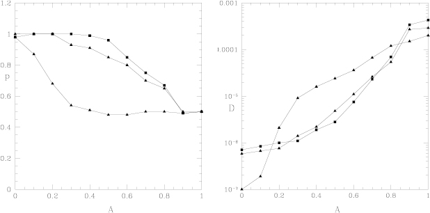
Figure 5. Asymptotic ITER ion transport fit by  . Plots of
  (left) and
  (right) versus
  . The lowest curves for
  are for 1 keV ions with
  and
and  (triangles), and the upper curve is for 10 keV ions with
  (squares), with
  the toroidal transit time. The constant
  is somewhat different, increasing dramatically with
  for 1 keV ions with
  to above the values for
  (triangles) and that for 10 keV ions (squares) over much of the range of
  .
.
Download figure:
Standard image High-resolution imageIn general, as the perturbation amplitude is increased, at some point the orbits become stochastic enough that the transport returns to be diffusional, with  . We cannot observe this transition in this system because the limited size prohibits evaluations for larger mode amplitudes. To this end we also examined a more uniform level of stochasticity in a simple circular equilibrium with
  using many small islands of uniform width, with
  and
and  , for which the stochastic orbit threshold was approximately constant across the plasma. In this case a long domain of amplitude with subdiffusive transport with
  was observed, followed by an abrupt return to normal diffusion with
  , at a perturbation level about three times the amplitude of the stochastic threshold. This is the amplitude at which the random phase approximation becomes valid.
2.2. Electrons
For electrons we carried out the same simulations using the ITER equilibrium consisting of  toroidal transits, or 70 ms, using energies of 10 keV and fairly large collision frequency, with
  , giving
  collision times. Large times were necessary because of the very small values of the transport. Electrons achieve subdiffusion for remarkably small values of the perturbations, well below values allowing a uniform representation in terms of stochastic properties. In figure 6 is shown the approach to subdiffusion (
 ) for very small values of mode amplitudes, and the values of the associated constant
  . The constant
  increases linearly with
  for all values, but much more slowly in the subdiffusive regime. Shown in figure 7 is the determination of 10 keV electron transport in ITER with mode amplitudes of
  (
( ) and
) and  (
( ), and the initial and final particle distributions for a simulation of
  transits. The initial domain is barely exceeded, transport is so slow that most of the particles remain within the original domain. Most of the domain covered by the particles consists of good KAM surfaces, but of course there are very small resonances, not visible in a large scale Poincaré plot, still influencing the electron orbits.

Figure 6. Asymptotic ITER electron transport fit by  . Plots of
  (left) and
  (right) versus
  for 10 keV electrons with
  . The constant
  increases monotonically with amplitude
  , but much more slowly after subdiffusion is attained.
Download figure:
Standard image High-resolution image
Figure 7. Determination of 10 keV electron transport in ITER with mode amplitudes of  (
( , lower) and
  (
( , upper) (left), and initial and final ITER electron distributions after
  toroidal transits for
  (right).
Download figure:
Standard image High-resolution imageThe units of  are in terms of poloidal flux and transit time. At
  we have
  in these units. Using the transit time of
  s, and noting that for electrons
  is approximately the poloidal flux, and using the electron gyro radius of
  cm, we find this value agrees with the Pfirsch–Schlüter value of diffusion of
  , giving approximately 7 cm
 s
s . Note from figure 1 that
  is very near 1. In the opposite limit,
  , transport is of the order
  m
m s
s , which is as large as the typical value of a turbulent diffusion coefficient in a tokamak [35]. This is not surprising, since we are considering a disruptive phase in ITER, not a typical tokamak transport case.
There are many publications concerning electron heat flux in stochastic fields, especially associated with a particular choice of equilibrium for ITER, called the CYCLONE [36] base case. Wang et al [37] use a simple enumeration of resonance islands and separations along with associated Poincaré plots to estimate proximity to stochastic threshold for a spectrum of 16 toroidal modes. They find the approximate stochastic threshold in this manner, but there now exist much more powerful methods to discover this [38, 39]. They then follow electrons for a total of 3000 toroidal transits. With levels of fluctuations such as shown in their plots probably one can fit the transport to  or to
or to  with equal accuracy. In addition, the Poincaré plots are made for zero frequency, valid for estimating the stochastic threshold for transport only provided the electrons can make very many toroidal transits in one mode period and in one collision time. Diffusion is assumed, but since the spectrum is very near stochastic threshold it is not clear this is warranted. In addition they refer to an exact relation between the magnetic field diffusion coefficient and associated electron heat flux, given by Harvey et al [40], but this paper again assumes that the field lines diffuse radially, making use of the random phase approximation used previously to calculate electron diffusion in a stochastic field [9].
3. NSTX
We examine discharge 141711 in NSTX at a time of 470 ms. In figure 8 are shown the equilibrium and the  profile. This discharge provides an example in which unstable Alfvén modes grow to a level which modifies the particle distribution without significant change in mode frequency, and with amplitudes which permit the use of linear eigenfunctions. Ten modes observed were analyzed by NOVA, given in [41].

Figure 8. NSTX equilibrium (left) and  profile (right).
Download figure:
Standard image High-resolution imageThe frequency of the modes is around 100 kHz, and the transit time for a 2 keV electron is  s, so an electron explores 50 toroidal transits in one mode period, enough to explore the intricacies of the field structure. On the other hand ion velocity is too small to explore the field structure in one mode period, and ion transport was found to be diffusive for all amplitude values.
In figure 9 are shown the mode harmonics as well as a plot of the mode amplitudes versus the poloidal mode number  . In the case of NSTX there are very few modes with amplitude above one tenth of the maximum amplitude mode. Large amplitudes are seen for
  , with smaller contributions with
  ,
,  , and
, and  .
.

Figure 9. Mode harmonics for TAE modes in NSTX (left) and the mode amplitudes as a function of the poloidal mode number,  (right).
Download figure:
Standard image High-resolution imageIn figure 10 is shown the transport fit to  for 2 keV electrons as a function of mode amplitude. Electrons are seen to make a fairly rapid transition to subdiffusive behavior at about the experimentally observed mode amplitudes,
  . In addition, the often quoted value of
  is not what is observed. At the transition the transport quickly changes to
  and then after this drops to
  just before the onset of complete stochastic loss. In figure 10 the determinations of the value of
  are shown for
  , for
, for  , and for
  . Values much above
  cannot be obtained, the amplitudes are such that the particles are lost before a reasonable determination can be made.
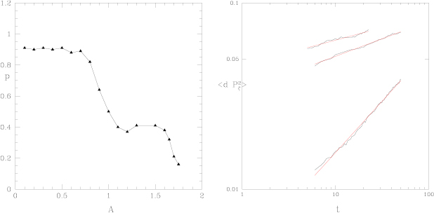
Figure 10. Asymptotic transport fit by  for 2 keV electron transport for TAE modes in NSTX. Plot of
  versus
  (left), and plots for
  with
with  (lower),
  with
with  (middle), and
  with
with  (upper).
Download figure:
Standard image High-resolution image4. ASDEX Upgrade
Now we consider ASDEX Upgrade (AUG) [24] in a state leading up to a disruption, the pre-disruptive phase of the L-mode, high density shot 30984, at  s. The shot was part of a campaign aimed at avoiding disruptions by applying electron cyclotron heating at the
  resonance [42, 43], and some evidence was found in the past of a role of magnetic field stochastization in forming the path to a disruption in AUG [44]. A still open question is the role of the
  island, as opposed to magnetic chaos in the outer part of the plasma, in the thermal quench preceding the disruption. The equilibrium and
  profile are shown in figure 11, and the tearing mode harmonics in figure 12. The harmonic content consisted of a single mode with
  and
and  , and the frequency was 1.7 kHz. Eigenfunctions are described as three-parameter functions, customarily used in AUG to match the
  island width with ECE measurements [45]. In our case study, the eigenfunction amplitudes and phases were matched to the measurement of amplitude and phase of the
  signal, as measured by the in-vessel C09 pick-up probes: given the equilibrium at a given time instant, eigenfunctions are then determined through a simple matrix inversion. Still some indeterminacy is present (especially for the high-
 numbers), due to the well-known pollution of the pick-up probe signal by means of the in-vessel passive structures, primarily the passive stabilization loop (PSL) [46]. The complete removal of the pollution is still work in progress: but in the present study we are interested in a general feature of transport, and in a parametric study similar to that shown previously for ITER, we will show that the main message of the analysis does not change, i.e. that transport is subdiffusive.

Figure 11. AUG equilibrium (left) and  profile (right),
  kG on axis.
Download figure:
Standard image High-resolution image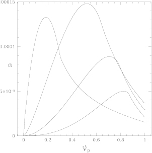
Figure 12. AUG harmonics in a pre disruptive state, consisting from left to right, of  , all with
  . Mode frequency was 1.7 kHz.
Download figure:
Standard image High-resolution imageThe Poincaré plot shown in figure 13 was made with co-passing collisionless electron orbits all with  , to show the nature of the resonances. Clear resonance islands are seen for each harmonic, as well as a nonlinearly generated resonance at
  . The position of the
  island agrees broadly with that measured in similar discharges [42] (note that in the AUG case the Poincaré is plotted with
  on the
  -axis, which, taking into account Orbit normalization and the fact that
  , coincides with the usual tokamak
  ).
).
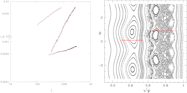
Figure 13. AUG electron diffusion at different locations in the device. For  the transport was superdiffusive with
  , shown in the middle curve on the left, with the final particle distribution shown with a horizontal line in the Poincaré plot at
  . Particles launched at
  exhibited subdiffusive transport with
  . Shown with the lower data on the left, with the final particle distribution shown with a horizontal line in the Poincaré plot at
  . Particles launched at
  are within the stochastic domain existing outside the
  surface and the transport was subdiffusive with
  , shown with the upper data on the left, with the final particle distribution shown with a horizontal line in the Poincaré plot at
  .
.
Download figure:
Standard image High-resolution imageTo study transport 300 eV electrons were launched with a uniform pitch distribution, a fixed initial flux surface, and a given pitch angle scattering rate. They were followed for a time of 3000 toroidal transit times, corresponding to 30 collision times. Transit time for an electron is this configuration is 1  s, so the particles were followed for 3 ms. The data for the evolution of the canonical momentum
  was necessarily truncated by discarding the initial ballistic motion and in some cases also the final points because particles had reached the boundary of the device.
We chose three different initial surfaces. Particles launched at  are within the resonance island produced by the
  and in this region the transport was superdiffusive with
  , due to the large excursions in the
  resonance. The points in the plot of
  are clearly seen to be those with the largest slope. The final extent of the particle distribution for this case is shown with a horizontal line at
  , seen to occupy the entire range of this resonance. Particles launched at
  are near the nonlinearly produced
  resonance, but where many good KAM surfaces also exist, and in this region the transport was subdiffusive with
  . In the plot of
  in addition to the small slope this trajectory also has a very small value of transport. The final extent of the particle distribution is also shown with a horizontal line at
  . Particles launched at
  are within the stochastic domain existing outside the
  surface and in this region the transport was subdiffusive with
  , and with a much larger coefficient than observed at
  . The final extent of this particle distribution is also shown with a horizontal line at
  , and occupies the entire stochastic domain outside the
  surface. It is interesting to note that the large
  resonance, with no apparent stochasticity nevertheless produces much stronger electron transport than does the stochastic domain, the island effectively providing rapid mobility across it. This confirms the traditional picture that the
  island has a fundamental role in the thermal quench preceding disruption, despite the weak chaos which dominates the outer part of the plasma.
We also investigated the dependence of the transport on the amplitude of the perturbations. The result is shown in figure 14. The values of  are shown for the three launch locations,
  for the amplitudes shown in figure 12 multiplied by 0.6, and 0.8 and 1.0. The results are remarkably independent of this change in mode amplitude, the only difference observed is that for amplitude reduction by 0.6 (squares in figure 14) the value at
  is even larger than the other determinations, with
  larger than 2.

Figure 14. Transport determination for different mode amplitudes as a function of initial particle position: triangles ( ) correspond to
  and 1, while squares (
 ) correspond to
  .
.
Download figure:
Standard image High-resolution image5. RFX
The Rechester–Rosenbluth (RR) formalism [9] is often used to describe energy and particle transport in the reversed-field pinch, and in particular in the RFX device in Padova [14]. The RR theory in the RFP is complemented with the Harvey equation for particle and energy transport [40] and a diffusive-convective scheme for the fluxes (Fick's law) in the form  . Yet, the RR theory would predict a particle diffusivity scaling
  with the normalized tearing mode amplitude, which corresponds to an energy confinement time scaling
  . On the contrary, experiments show a scaling
  for the diffusivity [47] and a different scaling for the energy confinement time
  [48]. We will demonstrate that both results, the exponent
  for the diffusivity scaling, and the inconsistency with the energy confinement scaling, are signatures of a subdiffusive nature of transport. In a preceding work [8] we have already shown that ion transport in the RFX is subdiffusive, with exponent
  . If one sticks with a diffusive-convective scheme, a phenomenological
  can be still obtained from a steady-state local density evaluation with Orbit (see [8] for details): in this sense, the term
  ('pinch' velocity) in the Fick's law
  can be interpreted as the subdiffusive correction to the diffusive evaluation of the fluxes. In these simulations, tearing-mode eigenfunctions are obtained from the 3D magnetohydrodynamic (MHD) nonlinear, visco-resistive cylindrical code SpeCyl which computes a chaotic, multiple-mode RFP state at Lundquist
  and Prandtl number
  [49]. This chaotic state is often called multiple helicity (MH) state. Modes with
  and
and  are considered. Test particles are ions at thermal energy
  keV and normalized collision frequency
  (2.5 toroidal transits per collision time). Eigenfunctions (
 and
and  ) and corresponding Poincaré map for this MH state of the RFP are shown in figure 15. The overlapping of the magnetic islands which resonate at several radii (
 in the RFP case) produces a large chaotic domain which anyway is full of hidden structures (cantori, as explained in the introduction [12, 50]) which are at the root of the subdiffusive behaviour in this system [8]. For example,
  ,
,  and
and  islands are still visible amid the chaotic sea in figure 15(b). Moreover, conserved islands with
  are always found in the RFP edge at the
  surface [51].

Figure 15. ( ) RFX harmonics for a MH, chaotic reversed-field pinch configuration. Modes have
  and
and  : only some
  's are considered in the plot; (
 ) Corresponding Poincaré map, showing a broad, chaotic region in much of the plasma volume, with some conserved structures, such as the
  ,
,  and
and  islands. Note the large conserved
  island in the plasma edge, which is responsible for a great part of the plasma confinement.
Download figure:
Standard image High-resolution imageThe scaling of the  values with the normalized mode amplitude is shown in figure 16.
  and
and  increase together as a function of the mode amplitude, which is usually interpreted in the RFP as a 'confirmation' of the Harvey theory, since also in the derivation of the pinch velocity from the kinetic equations made by Harvey [40],
  and
and  are proportional. But the fact that the exponent
  in Orbit ion simulations is a clear signature that something different is happening. This is made clear if one plots the ion flux,
  , as a function of
  . This is shown in figure 17: the flux scales with the mode amplitude even better that
  , but with a different exponent
  ! We can interpret the result in this way:
  shows that the magnetic field is far from being fully stochastic, with uniform and isotropic chaos. As a consequence, transport is subdiffusive. If transport is subdiffusive, the total flux
  must be corrected (at first order) with the 'pinch' velocity, and as a consequence the scaling for
  is different from the scaling for
  , as observed experimentally [47, 48]. The exponent
  found for the ion flux in Orbit simulations is very close to the experimental value
  of the exponent for
  , experimentally determined in a large RFX database [48].

Figure 16. ( ) Diffusion coefficient
  and (
and ( ) 'pinch' velocity
  as a function of the normalized mode amplitude
  .
.  and
and  are obtained through a least-squares fit of the local density distributions, as explained in [8]. The solid, red line in (
 ) represents a fit of the RR formula.
Download figure:
Standard image High-resolution image
Figure 17. Ion flux  as a function of the normalized mode amplitude
  . The solid, red line represents the least-squares fit.
Download figure:
Standard image High-resolution imageWe can repeat the analysis done for ITER and NSTX, by considering the asymptotic behaviour of particle transport as a function of time. This is shown in figure 18 by plotting the value of the radial spreading  as a function of time and averaged over the particle distribution. In panel (
 ) in the same figure, the value of the toroidal angle
  is shown. Particles are 10 000 ions at thermal energy
  keV and normalized collision frequency
  (the same as in figures 16 and 17), initially deposited at
  . Tearing mode amplitude in this case is fixed at
  , which is a typical case for RFX [8]. Particles are followed for 1600 toroidal transits. In figure 18(a) it is evident that, after a short, ballistic behaviour, particles show a clear, radial subdiffusive transport with exponent
  . When motion in the angle
  becomes diffusive (see panel (
 )), even stronger subdiffusion is reached, with
  . After ∼
 toroidal transits, many particles hit the wall, and
 ![$ \newcommand{\mean}[1]{{\langle #1 \rangle}} \mean{\Delta r^2}$](https://content.cld.iop.org/journals/0029-5515/59/1/016019/revision2/nfaaf07cieqn329.gif) saturates. The presence of a diffusive regime in the angle
saturates. The presence of a diffusive regime in the angle  after a few toroidal transits is due to the fact that, at longer timescales, collisions become important in reversing direction along the field, making the toroidal motion diffusive [8] (this is consistent with the collision frequency
  ).
).

Figure 18. Ion transport in a typical, chaotic state in the RFX reversed-field pinch: ( ) the value of
  as a function of time and averaged over the particle distribution; (
 ) the same for the toroidal angle,
  .
.
Download figure:
Standard image High-resolution imageWe can finally check the persistence of subdiffusion as a function of collision frequency: in figure 19 the asymptotic fit of ion transport ![$ \newcommand{\mean}[1]{{\langle #1 \rangle}} \mean{\delta r^2} = D t^{\,p}$](https://content.cld.iop.org/journals/0029-5515/59/1/016019/revision2/nfaaf07cieqn336.gif) is shown for different values of
is shown for different values of  , in the range
  . Diffusivity is rather large if compared with tokamaks,
  m
m s
s , but it is compatible with the local evaluation of figure 16 and with previous estimates, both experimental [47] and theoretical [52]. The most striking result is that transport remains subdiffusive in a broad range of collision frequency, with
  for
for  . Since the RFX experimental range of H
 collisions is
  , this means that ion transport is always subdiffusive in this device. Just from an academic point of view, ion transport would turn diffusive,
  , for
, for  , which would correspond to the fully collisional, Pfirsch–Schlüter regime, which can be accounted for in RFX only with heavy impurities [52].

Figure 19. Top: values of  in RFX as a function of normalized collision frequency
  for ion transport; bottom: the same for the exponent
  .
.
Download figure:
Standard image High-resolution imageSimilarly, we can analyze the values of  and
and  in the case of electrons: this is shown in figure 20. The collisional range is
  , since
  is rarely attained for electrons in the RFX device. Electron transport is even more subdiffusive in the whole collisional range, with
  for typical RFX electron collision frequency. The values of
  are in the range
  –
– m
m s
s , quite large: it should be noted that anyway the ambipolar
  , since a strong ambipolar potential develops in the RFX to balance a too strong electron diffusion [53]. Finally, it is noteworthy that subdiffusion in the RFX appears at a relatively modest level of perturbation amplitude,
  %.
%.

Figure 20. Top: values of  in RFX as a function of normalized collision frequency
  for electrons; bottom: the same for the exponent
  .
.
Download figure:
Standard image High-resolution image6. DIII-D
Deuterium beam ions in  plasmas drive the instability of many toroidicity-induced Alfvén eigenmodes (TAE) and reversed shear Alfvén eigenmodes (RSAE). The mode structure is measured with electron cyclotron emission (ECE) and beam-emission spectroscopy (BES) diagnostics. Saturated mode amplitudes are derived by scaling the prediction of a synthetic ECE diagnostic applied to NOVA calculated eigenfunctions. The resultant beam-ion transport is measured by five independent techniques [54–56], including spatially-resolved fast-ion D-alpha (FIDA) spectroscopy. The data imply strong central flattening of the fast-ion profile during the early phase of the discharge when many Alfvén modes are unstable. In figure 21 are shown the equilibrium and the
  profile.

Figure 21.  equilibrium and
  profile.
Download figure:
Standard image High-resolution imageWe used NOVA calculated eigenfunctions that were experimentally validated by ECE measurements with the guiding center code Orbit [20, 57]. The modes were localized near the plasma core, producing a flattening of the distribution, but no induced particle loss. In figure 22 are shown the modes and a plot of mode amplitudes. DIIID has a wider spectrum of modes than does NSTX. There are 8 different modes with n values ranging from 1 to 5, and frequencies ranging from 62 kHz to 80 kHz with a total of 105 poloidal harmonics.

Figure 22.  harmonics. There are many harmonics present with comparable amplitudes, with
  between 20 and 100.
Download figure:
Standard image High-resolution image
In this case the mode spectrum is broad enough to produce diffusion of ions and electrons for all mode amplitudes. There is no transition to strong subdiffusive behaviour observed for either species. The spectrum of  values is very different from the case of NSTX. This spectrum is uniform enough to make the random phase approximation valid, and to preclude strong subdiffusion, justifying the use of a diffusion model, employed in analyzing the effect of modes on the beam profile [56].
7. Conclusion
This paper presents a detailed study of transport in toroidal plasma confinement devices in states approaching disruption, with a spectrum of saturated tearing modes, or with a spectrum of Alfvén modes. For perturbations leading up to plasma disruption in ITER subdiffusive transport is found for both ions and electrons for values of magnetic perturbations well below those producing a uniform level of stochasticity allowing more general methods of evaluation, and for mode amplitudes for which a large scale Poincaré plot of the orbits appears to consist of well defined KAM surfaces. In general ions are strongly affected in pre-disruption states, but not generally by spectra of Alfvén modes, because the high frequency makes the perturbation effectively random before an ion can complete a sufficient number of toroidal transits. Electron transport can become subdiffusive for surprisingly small amplitudes and even for high frequency perturbations, depending on the nature of the mode spectrum. The exact nature of the perturbed field is important not only for the precise value of the nondiffusive transport, but also for its existence. Low level field perturbations can produce complicated structure (Markov tree of cantori [12]) giving rise to long time correlations and local traps, and significantly modify particle transport, but if the mode spectrum is sufficiently broad and uniform, as seen in  , the transport can be diffusive for all mode amplitudes. Note that the kick model [58] for the modification of particle distributions due to Alfvén modes makes no assumption regarding the nature of the transport.
In many cases the observed subdiffusive transport closely approaches the classically given  , but we also find exceptions to this, with different fractional powers of
  . In RFX the subdiffusive transport leads to an understanding of the energy confinement time and diffusivity scaling with the perturbation amplitude.
In conclusion, it is shown that the ubiquitous use of a diffusive scheme to predict and analyze electron and ion transport in toroidal plasmas is not justified in the main scenarios of some important confinement devices, and that extrapolations based on diffusive models lead to incorrect and often misleading results.
Acknowledgment
This work was partially supported by the U.S. Department of Energy Grant DE-AC02-09CH11466. This material is based upon work supported by the U.S. Department of Energy, Office of Science, Office of Fusion Energy Sciences, using the DIII-D National Fusion Facility, a DOE Office of Science user facility, under Awards DE-FC02-04ER54698. DIII-D data shown in this paper can be obtained in digital format by following the links at https://fusion.gat.com/global/D3D_DMP. This report was prepared as an account of work sponsored by an agency of the United States Government. Neither the United States Government nor any agency thereof, nor any of their employees, makes any warranty, express or implied, or assumes any legal liability or responsibility for the accuracy, completeness, or usefulness of any information, apparatus, product, or process disclosed, or represents that its use would not infringe privately owned rights. Reference herein to any specific commercial product, process, or service by trade name, trademark, manufacturer, or otherwise does not necessarily constitute or imply its endorsement, recommendation, or favoring by the United States Government or any agency thereof. The views and opinions of authors expressed herein do not necessarily state or reflect those of the United States Government or any agency thereof. One author (RW) acknowledges useful collaborations with W.W. Heidbrink, C.S. Collins, and M.A. Van Zeeland. Another author (GS) thanks S. Cappello, M. Veranda and F. Auriemma for suggestions and corrections to the manuscript, and the whole RFX-mod team for continuous support. This work has also been carried out within the framework of the EUROfusion Consortium and has received funding from the Euratom research and training programme 2014–2018 under grant agreement No 633053. The views and opinions expressed herein do not necessarily reflect those of the European Commission.