

Abstract
Objective. The goal of this study was to develop a physiologically plausible, computationally robust model for muscle activation dynamics (A(t)) under physiologically relevant excitation and movement. Approach. The interaction of excitation and movement on A(t) was investigated comparing the force production between a cat soleus muscle and its Hill-type model. For capturing A(t) under excitation and movement variation, a modular modeling framework was proposed comprising of three compartments: (1) spikes-to-[Ca2+]; (2) [Ca2+]-to-A; and (3) A-to-force transformation. The individual signal transformations were modeled based on physiological factors so that the parameter values could be separately determined for individual modules directly based on experimental data. Main results. The strong dependency of A(t) on excitation frequency and muscle length was found during both isometric and dynamically-moving contractions. The identified dependencies of A(t) under the static and dynamic conditions could be incorporated in the modular modeling framework by modulating the model parameters as a function of movement input. The new modeling approach was also applicable to cat soleus muscles producing waveforms independent of those used to set the model parameters. Significance. This study provides a modeling framework for spike-driven muscle responses during movement, that is suitable not only for insights into molecular mechanisms underlying muscle behaviors but also for large scale simulations.
Export citation and abstract BibTeX RIS
1. Introduction
The muscle is a fundamental element in mammalian motor systems that produces the force to make proper movement. The workflow of the muscle force has been known to be collectively shaped through a pool of motor units, which consists of a motoneuron in the spinal cord and muscle fibers that it innervates (Burke et al 1973, Zajac and Faden 1985). Computational approaches have been applied to gain insight into the relationship between neural input and force output at the motor system level (Fuglevand et al 1993, Williams and Baker 2009, Elias et al 2012), partially due to the difficulty in simultaneously accessing the motoneuron pool and its muscles during movement in humans and animals (Heckman and Enoka 2012). However, muscle responses in previous simulation studies have been represented phenomenologically for input conditions limited to steady neural excitation and isometric muscle contraction. Therefore, to accurately understand the input–output properties of a neuromuscular system under more natural input conditions, the previous phenomenological and static muscle models must be extended to reflect nonlinear muscle behaviors that have been experimentally observed during dynamic variations in excitation and movement (Brown et al 1996, Brown et al 1999, Rassier et al 1999) and to be implementable on the same platform of neuron simulators (e.g., NEURON or GENESIS) where motoneurons can be anatomically reconstructed and physiologically simulated for biological realisms (De Schutter 1992).
The Hill-type model of muscle and tendon is the most widely used approach to estimate force production in many large-scale simulations of human posture and movement. This is due to the ease of implementation, simplicity of its formulation, and direct relationship of its parameters to experimental measures of force–velocity and length–tension (L–T). (Zajac 1989, Gerritsen et al 1996, Sartori et al 2012). However, direct comparisons of Hill-type models and actual muscles have revealed that Hill-type models may not have sufficient accuracy for dynamic changes in both excitation frequency and muscle length (Sandercock and Heckman 1997b, Millard et al 2013, Perreault et al 2003). Simulation errors have been reported to be prominent, particularly over the sub-maximal excitation frequency range (≤20 Hz) during the random movement representing locomotion. Results from these comparison studies have reinforced the idea that the dynamics of muscle activation strongly depend on excitation frequency and muscle movement in dynamic conditions.
Predicting the activation dynamics of Hill-type models is difficult, hindering the advancement of realistic simulations of neuro-musculo-skeletal models under physiological input conditions (Campbell 1997, Tanner et al 2012). Under certain conditions, activation dynamics have been estimated either indirectly based on raw electromyography (EMG) data recorded from the muscle of interest (Thelen et al 1994, Lloyd and Besier 2003) or directly by solving the Huxley formulation that describes the spatiotemporal interactions of the thin and thick myofilaments forming cross-bridges in the sarcomere (Wong 1971, Laforet et al 2011). Although EMG-based models could be implemented with relative ease using a small number of model parameters, they may sacrifice insights into the biophysical mechanisms underlying the activation dynamics because they concentrate on the overall performance of a muscular system. In contrast, cross-bridge (or Huxley-type) models may provide a framework for mechanistically modeling muscle activation, but the stiff nature of their system equations has increased computational cost and a stability issue in numerically solving the equations in particular while varying model parameter values over a wide range (Zahalak 1981, Zahalak and Ma 1990). In this study, we aimed at developing a dynamical model for muscle activation that is biophysically plausible and practically robust over a wide range of physiological input conditions, such as for excitation frequency and muscle length.
For this goal of the study, we first investigate how the excitation and the movement interact on the dynamics of muscle activation: dependencies of the activation dynamics on muscle movement and excitation frequency are identified by comparing the actual data obtained from a cat soleus muscle with its Hill-type model for both static and dynamic variation in the excitation frequency and muscle length. To incorporate the excitation and movement dependencies of the activation dynamics, we then present a novel modeling approach that allows for the prediction of the activation dynamics of Hill-type muscle models driven by electrical impulses (or spikes) during physiological movement. The signal transformations of the electrical spikes in the sarcoplasm for producing force are modeled in a modular form so that the model parameter values are determined by an individual module based on experimental data obtained under static conditions (i.e., isometric and isokinetic). Finally, the modified Hill-type model compensating for the dependencies of the activation dynamics on the frequency and length was validated using waveforms independent of those used to set the model parameters for cat soleus muscles. The nonlinear muscle behaviors that the proposed modeling approach may not cover and the further works needed to build the population model of heterogeneous motor units are discussed for future studies.
2. Methods
2.1. Experiments
Data for an average input–output properties of S-type muscle units were collected from the left hindlimb soleus muscles of two adult cats. The data set obtained from one cat (CT09) was used for developing the new modeling framework, whereas the same data set independently measured from another cat (CT95) was used to validate that the developed modeling approach can be utilized as a template for modeling soleus muscles. All procedures were approved by the Animal Care Committee at Northwestern University. Details of the surgical preparations and experimental protocols have been previously reported (Sandercock and Heckman 1997b, Perreault et al 2003).
Briefly, cats were anesthetized with isoflurane (1.5–3.0%), the soleus muscle was exposed, and the distal tendon was attached to a computer-controlled puller. All distal hindlimb nerves except the soleus nerve were disconnected. Only ipsilateral dorsal roots from L4 to S2 were transected to eliminate sensory feedback from the soleus. Decerebration was performed at the midbrain level. Hindlimb and core temperatures were maintained within physiological limits using radiant heat. At the end of the experiment, animals were euthanized with pentobarbital (100 mg kg−1 i.v.).
Electrical impulses with 0.1 ms width were generated by a square pulse stimulator (Grass S88; Natus, Middleton, WI) and applied for controlling muscle force either using fine stainless steel wires in the proximal and distal portions of the muscle belly or via hook electrodes on the ventral roots. Similar results were obtained with both methodologies. The full recruitment was assessed by reaching a plateau with increasing current intensity. A supra axial current (50–100% above that required to elicit full recruitment) was used to produce repeatable and consistent forces during all trials.
Muscle length was controlled by a position servo system, which is a computer-controlled muscle puller (AV-50; ADI, Alexandria, VA). This device had a stiffness of greater than 60 kN m−1 and a small signal position bandwidth of approximately 50 Hz. Muscle length was measured by a linear variable differential transformer (500 dc-B; Shaevitz, Hampton, VA) attached to the puller shaft. Muscle force was measured by a strain gage-based transducer (Model 31 (stiffness >2 MN m−1); Sensotec, Columbus, OH) in series with the shaft. Force and position data were sampled at 1 kHz (MIO-16; National Instruments, Austin, TX). In order to isolate the active force response, we subtracted the force data measured without the stimulation (i.e., passive response) from that measured with the stimulation (i.e. active response) under the same condition of muscle length. The passive and active trials were separated by a 30 s rest period and all active trials were also separated by at least one minute to minimize fatigue.
The active muscle force was recorded using five experimental protocols while ensuring that the interval (at least 1 min) between trials was sufficiently large to prevent fatigue: (1) twitch response at muscle lengths (−16, −8, and 0 mm for the CT09 and −10, −5, and 0 mm for the CT95), (2) sub-tetanic response with constant excitation frequencies (10, 20, and 40 Hz for both CT09 and CT95) at each muscle length, (3) L–T and velocity-tension (V–T) properties under full excitation (100 Hz for both CT09 and CT95), (4) step shortening of muscle length (0.5 mm for CT09 and 2 mm for CT95) during isometric contraction with full excitation to estimate the stiffness of the serial elastic (SE) component of the muscle, and (5) random modulation of the muscle length between −16 and 0 mm and excitation frequency with means of 10, 20, and 30 Hz for both CT09 and CT95.
Random variations in muscle length were produced with a bandwidth ranging from 0 to 5 Hz, matching the soleus length changes that occur during unrestrained locomotion (Goslow et al 1973). The time course of the muscle length was generated in two steps: random numbers were created in a white uniform 10 kHz sequence using a random number generator and then filtered with a low pass FIR filter using a Blackman window. All length perturbations were centered about an operating point −8 mm less than the physiological maximum length (0 mm). Stimulus trains had constant and uniformly distributed random interpulse intervals spanning a range between 0.01 s and twice the desired mean interpulse interval (0.10, 0.05, and 0.033 s).
2.2. Model construction
2.2.1. Modular modeling framework
The muscle model for force production in response to electrical spikes (i.e., neural commands) under movement consisted of three sub-modules (figure 1). We have chosen the mechanistic modeling approach not only for understanding the biological process underlying the muscle activation dynamics but also for extrapolating beyond the observed conditions by modulating model parameters such as rate constants (Williams et al 1998, Laforet et al 2011). The individual modules captured the biophysical characteristics of three signal transformations that the neural inputs undergo for force production. The electrical spikes in the model were first transformed into the concentration of free Ca2+ (CaSP) and Ca2+ bound to troponin (CaSPT) in the sarcoplasm in the first module (referred to as Module ①). Then, the second module (referred to as Module ②) transformed the CaSPT concentration from Module ① to the level of muscle activation (A(t)). Finally, the A(t) in Module ② was transformed to the force in the third module (referred to as Module ③). During the movement, the muscle length (Xm) information were fed into all of the model's individual modules.
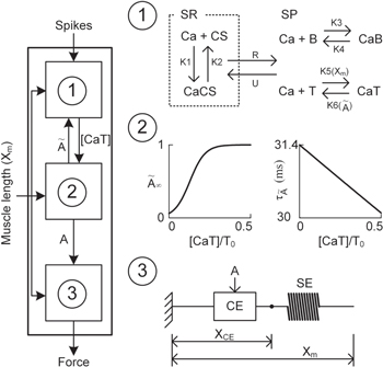
Figure 1. Schematic diagram of the modular muscle model. Three sub-modules (①, ②, and ③) on the left and the activity of the individual modules on the right. ① for calcium (Ca) dynamics in the sarcoplasm (SP) and the sarcoplasmic reticulum (SR) in response to electrical impulses. ② for activation dynamics (A(t)) governed by the steady-state relationship between the concentration of Ca bound to troponin ([CaT]) and  and the time constant (
 underlying the kinetics of reaching
  where
where  is further updated to A in exponential form as
  ③ for force production based on Hill mechanics in response to A.
Download figure:
Standard image High-resolution imageModule ①: the dynamics of the CaSP and CaSPT concentration in the sarcoplasm were modeled simplifying chemical reactions experimentally identified from single mouse muscle fibers in a previous study (Westerblad and Allen 1994). This module has two compartments: one for the sarcoplasmic reticulum (SR), containing free calcium ions (CaSR) and calsequestrin (CS), and the other for the sarcoplasm (SP), containing the free calcium ions (CaSP), free calcium-buffering proteins (B), and troponin (T) of thin filaments (upper panel in figure 1). The CaSP concentration was determined by the release and reuptake of Ca2+ through the membrane of the SR as well as by the Ca-buffering mechanism and Ca–troponin binding in the SP. When the model is stimulated with electrical impulses, the release (R) of Ca2+ from the SR was calculated as a function of the CaSR concentration, whereas the uptake (U) of Ca2+ back into the SR was made as a function of the CaSP concentration. The CaSR concentration was regulated in the SR by the forward and backward rate constants (K1 and K2) governing the reaction kinetics between the CaSR and Ca2+ bound to CS (CaSRCS) following the state equations
where the square brackets indicate concentration, CS0 is the total concentration of CS, and R and U are mathematically modeled as

Here, Rmax is the maximum permeability of the SR, τ1 and τ2 are the time constants of the increase and decrease in permeability, respectively, i indicates each stimulation impulse, ti is the time of ith stimulation impulse, n is the total number of stimulation impulses, Umax is the maximal pump rate, and K is the site binding constant for Ca2+ to activate the pump in the SR.
The calcium ions released from the SR were further regulated by interaction with B and T in the SP. The kinetics of chemical reactions between these substances (CaSP, B, and T) were governed by four rate constants (K3–K6) following the state equations
where the square brackets indicate concentration, K3 and K4 are the forward and backward rate constants between the CaSP and Ca2+ bound to B (CaSPB), respectively, and K5 and K6 are the forward and backward rate constants between the CaSP and CaSPT, respectively. The cooperativity in the Ca–troponin binding during force development was reflected by making K6 a function of the muscle activation  for steady conditions, as previously reported (Westerblad and Allen 1994): K6 = K6i/(1 + 5 ·
  where K6i is the initial rate constant and
  is fed from the second module. B0 and T0 are the total concentration of B and T.
Module ②: the [CaSPT] in the sarcoplasm was transformed to the activation dynamics (A(t)) reflecting the cooperative formation of cross-bridges with increasing force (middle panel in figure 1). This cooperativity of cross-bridge formation has been characterized as a sigmoidal relationship between the sarcoplasmic Ca2+ concentration and force production under steady-state conditions (Shames et al 1996). In this module, the steady-state relationship between [CaSP] and the force was first mapped to that of [CaSPT] and the activation level ( for the steady Ca stimulation. Morris–Lecar formulation, including five parameters (C1–C5) (Morris and Lecar 1981), was chosen to dynamically represent the nonlinear [CaSPT]–
 relationship using the following equations

and
where  is the steady-state value of
 at the normalized [CaSPT] relative to the total troponin concentration (T0) in the SP,
  is the time constant controlling the speed at which the individual values of
  are approached, C1 is the normalized [CaSPT] for half muscle activation, C2 is the slope of the activation curve at C1, C3 is the scaling factor for temperature, C4 is the normalized [CaSPT] for the maximum time constant, and C5 determines the width of the bell-shaped
  curve.
Then, for the transient [CaSP] variation during electrical excitation, the  was updated to the A(t) in exponential form as
  with an exponent α assuming the reduction in the likelihood of the cross-bridge formation under the impulse stimulation relative to the steady case.
Module ③: given muscle activation (A), force was produced using the simplest form of Hill-based muscle models, which consists of two elements: contractile compliance (CE) in series with SE lumping tendon and aponeurosis compliances (Zajac 1989) (bottom panel in figure 1). The force output (F) was determined by the difference between the deviation in muscle length (ΔXm) and the contractile element (ΔXCE) from their initial lengths as

where P0 is the peak force at the optimal length and KSE is the stiffness of the SE element normalized by P0.
To calculate ΔXCE in equation (9) at various levels of muscle length and activation, the original equations suggested by Hill (Hill 1938) for shortening and Mashima (Mashima et al 1972) for lengthening were modified as

where a0, b0, c0, and d0 are Hill–Mashma equation coefficients, g(Xm) represents the L–T relationship of muscles as a Gaussian function (i.e., bell-shaped) normalized with the P0, and g1-g2 are Gaussian coefficients indicating the optimal muscle length and width of the curve. Equations (9)–(12) were also used to inversely estimate the activation dynamics (A(t)) of a given muscle force (F) and length (Xm) profile.
We have constructed a new modular framework for muscle modeling introducing Module ② to dynamically represent the [CaSPT]-A relationship resulting from the cross-bridge formation under variation in the input (excitation frequency and muscle length) conditions.
2.2.2. Determination of model parameter values
The parameter values of the new muscle model could be determined separately for the individual modules based directly on experimental data. In this study, all of the parameter values for Module ① were adopted directly from previously reported mouse experiments (Westerblad and Allen 1994).
The parameter values for Module ③ were then determined from data measured under three different conditions; (1) KSE in equation (9) was determined by dividing the force drop amplitude by the length step during the step-shortening experiment and normalizing this value by the maximal force at the optimal length (see figures S1A-S1B for the shape of the response to the length step); (2) the Gaussian coefficients (g1-g2 in equation (12)) were estimated from the L–T properties obtained from an actual muscle, where g1 was set to the optimal lengths (−8 mm for CT09 and −5 mm for CT95) and g2 was adjusted to cover the full range (0–16 mm for CT09 and 0–10 mm for CT95) of muscle length investigated in the experiment (see figure 3 for details of the L–T data); and (3) Hill–Mashma coefficients (a0–d0 in equations (10) and (11)) were analytically determined based on the V–T property of actual muscles by deriving inverse equations for the four coefficients given four data points ((VS,1, TS,1), (VS,2, TS,2), (VL,1, TL,1), (VL,2, TL,2)) on the V–T curve (see figure 3 and figure S1 for details of the V–T data):


where VS,1 and VS,2 are the minimum and maximum shortening velocities and VL,1 and VL,2 are the minimum and maximum lengthening velocities. The four data points measured to determine the four Hill–Mashma coefficients were (−160, 1), (−1, 22), (1, 23.5), and (80, 34.35) for CT09 and (−80, 8), (−1, 28), (1, 29.5), and (80, 43) for CT95, where the units are mm s−1 and N for velocity and tension, respectively.
Finally, the parameter values (C1–C5 and α) of Module ② were adjusted to match experimental data for twitch and sub-tetanus responses with an excitation frequency ranging from 1 to 40 Hz at the optimal length in the isometric condition (see figure 2(E) and figure S1 (available at stacks.iop.org/JNE/12/046025/mmedia) for details on the force data). The parameter values were optimized using the optimization tool (i.e., Multiple Run Fitter based on PRAXIS algorithm) built in the NEURON software (Hines and Carnevale 1997).
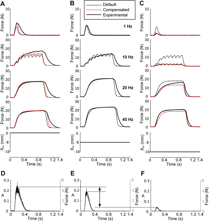
Figure 2. Twitch and sub-tetanic forces at various muscle lengths. (A)–(C), twitch and sub-tetanic responses of the actual muscle (CT09), the model with default parameter values, and the model compensating for the length dependence of A(t) using equation (18), at three muscle lengths (Xm) of 0 (A), −8 (B), and −16 mm (C) under constant excitation with frequencies of 1, 10, 20, and 40 Hz. (D)–(F), activation dynamics (A, dotted black lines) inversely calculated using equations (9)–(12) directly from the twitch responses (gray lines) measured at three different lengths: 0 mm (D), −8 mm (E), and −16 mm (F).
Download figure:
Standard image High-resolution imageAll steps were repeated for different sets of experimental data obtained from another cat preparation (i.e., CT95) to validate the proposed modeling approach. All parameter values and units used in this study are presented in table 1.
Table 1. Model parameters and values.
| Parameter | CT09 | CT95 | |
|---|---|---|---|
| Module ① | K1 (M−1 s−1) | 3000 | 3000 |
| K2 (s−1) | 3 | 3 | |
| K3 (M−1 s−1) | 400 | 400 | |
| K4 (s−1) | 1 | 1 | |
| K5 (M−1 s−1) | 4e5 | 4e5 | |
| K6i (s−1) | 150 | 150 | |
| K (M−1 s−1) | 850 | 850 | |
| Rmax (s−1) | 10 | 10 | |
| Umax (M−1 s−1) | 2000 | 2000 | |
| τ1 (ms) | 3 | 3 | |
| τ2 (ms) | 25 | 25 | |
| φ1 (mm−1) | 0.03 | 0.006 | |
| φ2 | 1.23 | 1.03 | |
| φ3 (mm−1) | 0.01 | 0.006 | |
| φ4 | 1.08 | 1.03 | |
| Module ② | C1 | 0.128 | 0.118 |
| C2 | 0.093 | 0.11 | |
| C3 (ms) | 61.206 | 68.319 | |
| C4 | −13.116 | −3.94 | |
| C5 | 5.095 | 1.368 | |
| α | 2 | 2 | |
| α1 | 4.77 | 2 | |
| α2 (ms) | 400 | 400 | |
| α3 (ms) | 160 | 160 | |
| β | 0.47 | 0.001 | |
| γ (s mm−1) | 0.001 | 0.001 | |
| Module ③ | KSE (mm−1) | 0.4 | 0.57 |
| P0 (N) | 23 | 28.9 | |
| g1 [mm] | −8 | −5 | |
| g2 (mm) | 21.4 | 27.5 | |
| a0 (N) | 2.35 | 0.18 | |
| b0 (mm s−1) | 24.35 | 31.31 | |
| c0 (N) | −7.4 | −9.19 | |
| d0 (mm s−1) | 30.3 | 31.86 |
Note: φ1–φ4 are the parameters of equation (18) for compensating the length dependency of A(t) in the static conditions. α1-α3, β, and γ are the parameters of equation (20) for compensating the dependencies of A(t) during movement. The definition of individual parameters and the procedure of determining parameter values were fully described in the section 2.
2.3. Identification of A(t) dependency on excitation and movement
The dependency of A(t) on excitation frequency and muscle length was investigated based on the indirect method that has been used in our previous studies (Sandercock and Heckman 1997b, Perreault et al 2003). This method utilizes only Module ③ in our modeling framework. Given the length and force data from the soleus muscle (CT09), A(t) for Module ③ was first estimated inversely from equations (9)–(12). Then, the force production was compared between the real and model muscle with the inversely estimated A(t) while varying the length to identify the movement dependency of A(t). For the excitation dependency of A(t), the above process was repeated at various levels of excitation frequency. In the present study, this indirect investigation was performed for the static (isometric and isokinetic) conditions. During the dynamic (movement) conditions, the muscle model compensating for the identified dependencies of A(t) during the static (isometric and isokinetic) conditions was compared with the force data obtained from the soleus muscle under the same excitation and movement condition. The profiles of A(t) inversely estimated for the dynamic conditions were presented in detail in our previous paper (Perreault et al 2003).
2.4. Numerical simulations
The new muscle model, consisting of the three sub-modules, was implemented using the Neuron MOdel Description Language in the NEURON software environment (version 6.1). NEURON has been used as a general platform for computer simulations of real neurons (Hines and Carnevale 1997). Applying the same stimulation protocols as those in the experiments, the model was simulated using a numerical integration method (cnexp) built in the NEURON with a fixed time step (0.025 ms) ensuring the stability and accuracy of simulations while varying parameter values in a wide range. The initial values of the [CaSR] and CS0 in the SR, and the B0 and T0 in the SP were set to 2.5 mM, 30 mM, 0.43 mM, and 70 μM, respectively, based on a previous experimental study (Westerblad and Allen 1994).
3. Results
Dependency of the muscle activation dynamics (A(t) in figure 1) on excitation (stimulation frequency) and movement (muscle length) was first investigated for twitch and sub-tetanic contractions at discrete lengths (i.e., isometric). After compensating the modified Hill model (figure 1) with the default parameter values (table 1) for the identified dependence of A(t) during the isometric contractions, we further evaluated the movement dependence of A(t) during tetanic contractions over a wide range of constant velocities (i.e., isokinetic). Then, we tested the model compensating for all of the identified dependencies of A(t) in the static conditions for the dynamic cases where the frequency and length dynamically varied. Finally, we validated the model compensating for the identified dependencies of A(t) under the dynamic conditions against the real data obtained from the different muscle preparation (CT95). The degree of the A(t) dependency and the effectiveness of the compensation mechanisms for the A(t) dependencies were quantitatively evaluated calculating the percent root mean square error (RMSE) normalized by the difference between the maximum and minimum real force,

where the subscript m and s, and N indicate measurement, simulation, and the number of samples considered for evaluation, respectively.
3.1. Twitch and sub-tetanic responses at discrete lengths
Figure 2 presents the twitch and sub-tetanic responses of the model and actual muscle to various frequencies (1, 10, 20, and 40 Hz) at three different lengths (−16, −8, and 0 mm) centered at the optimal length. The default values for the model parameters (table 1) were determined to match the force data (figure 2(B)) measured at the optimal length in the same muscle.
The force output of the model was underestimated when the lengths were greater than optimal length (figure 2(A), see figure 7(A) for NRMSE values), whereas it was overestimated when shortened (figure 2(C), see figure 7(B) for NRMSE values). To explicitly determine whether A(t) depends on the length, A(t) was inversely estimated from the twitch response (black dotted lines in figures 2(D)–(F)) of actual muscle at each length using equations (9)–(12). The degree of change in the amplitude of A(t) was more severe when reducing the length, rather than increasing it. This dependence of the activation amplitude on length was compensated for by making the forward rate constant (K5 in figure 1) of the Ca2+–troponin reaction a function of the length (Xm), as suggested in a previous study (Williams et al 1998):
where φ1–φ4 are determined using the polyfit function (based on least squares method) built in Matlab for the dataset {(φ(Xm), Xm)|(0.77, −16), (1, −8), (1.08, 0)}, in which the model matched the peak of the twitch response measured at the three lengths (figures 2(D)–(F)).
After compensating for the length dependency of A(t) in equation (18), the simulation error was dramatically reduced, particularly for physiologically relevant frequencies (≤20 Hz) below the optimal length (figure 2(C), see figure 7(B) for NRMSE values). At high frequencies (≥40 Hz), there was no significant difference in the force production regardless of the compensation for the length dependence. This suggests that under full excitation, the activation dynamics are not influenced by the constant change in the length over time (i.e., isokinetic condition).
3.2. Isometric–isokinetic–isometric contractions under full excitation
The length compensated model of A(t) (equation (18)) was then evaluated for the L–T and V–T properties of actual muscle under a fully excited state. To definitively assess whether length and velocity influence A(t) during full excitation, A(t) was inversely estimated from the tetanic response of actual muscle at the optimal length using equations (9)–(12) (figure 3(A)). Given the same input conditions, the force responses predicted from the inversely estimated A(t) using (9)–(12) were compared to actual muscle, and the model compensated for isometric contractions.

Figure 3. Length- and velocity-tension properties under full excitation. (A) Activation dynamics (A, dotted black line) inversely calculated using equations (9)–(12) directly from force data (gray line) measured at the optimal length (−8 mm) in response to a 100 Hz impulse current (bottom). (B)–(G) Time course of muscle forces driven by the inversely estimated A(t), simulated by the new model, and the actual data during isometric–isokinetic–isometric contractions. (H) Profiles of muscle length (Xm) and velocity applied for (B)–(G).
Download figure:
Standard image High-resolution imageFigure 3(B)–(G) presents a comparison of muscle forces between the inverse model (dotted black), the compensated model (dotted red), and actual muscle (solid black) (see also figure 7(C) for NRMSE values). Both the inverse and compensated models matched the time course of force development observed in actual muscle during various isometric–isokinetic contractions (figure 3(H)). The agreement in the tetanic responses between actual muscle and the inverse model suggests that A(t) is not influenced by length and velocity changes with full excitation under static (isometric and isokinetic) conditions. The similarity in force responses between the inverse and compensated models indicates that the A(t) in the compensated model was almost identical to that of the inverse model. This result suggests that Modules ① and ② in the compensated model may replicate the physiological activation dynamics for isometric–isokinetic contractions with full excitation and confirms the prediction made in the previous section that the length dependency of A(t) tends to be weakened with increasing frequency.
3.3. Force production under dynamic changes in length and frequency
Having identified the length dependency of A(t) under the static condition, we evaluated whether the compensation for the length dependency of A(t) by equation (18) was sufficient to predict force production under dynamic input conditions.
Figure 4 compares muscle force between the compensated model (dotted red) in the static condition and experimental data (solid black) from three levels (10, 20, and 30 Hz) of constant frequency during random variations in the length between −16 and 0 mm (bottom, figure 4). As previously reported (Perreault et al 2003), the compensated model overestimated the force much more at physiologically relevant frequencies (<20 Hz) compared to higher level of excitation (see figure 7(D) for NRMSE values). Over these low frequencies, the slowly decreasing force output induced by the movement resulted in a prominent factor contributing to the simulation error. Because no molecular mechanism underlying this movement-induced force reduction has been reported, we arbitrarily compensated for this activation dependency by adding a mathematical term to the exponent (α) of  so that the α gradually increases during movement,

Figure 4. Force production during dynamic variations in muscle length. Force responses of the actual muscle (CT09), the model compensated under static (equation (18)) and dynamic condition (equation (20)), at three levels of excitation frequencies (10, 20, and 30 Hz) under the same profile of the dynamic change in muscle length (Xm, solid black) and velocity ( solid gray) in the bottom. The vertical gray area indicates the range of the length and velocity over which the simulation error (the difference between dotted red and solid black lines) is the most intensified.
Download figure:
Standard image High-resolution imageThe three coefficients, α1, α2 and α3 in equation (19), were adjusted using the NEURON Multiple Run Fitter (based on PRAXIS) to best fit the data at all three levels of constant frequency during movement. Overall, sigmoidal increase of the level of α as a function of time (equation (19)) led to a dramatic reduction in simulation error at all levels of excitation frequency (figure 4, see also figure 7(D) for NRMSE values).
The simulation error was also found to be intensified when the length was lower than the optimal length during positive (i.e., lengthening) velocity contraction (see the vertical gray areas in figure 4). To compensate for this length and velocity dependency of A(t) during movement with a minimum number of additional parameters, we further scaled the activation level by adding length and velocity dependence to equation (19) as mathematically modeled

where φ(Xm) is the same function defined in equation (18) and Vm are the time derivative of Xm; β and γ were set to 0 for lengths longer than the optimal length or during the negative velocity movement.
Consequently the addition of the length and velocity dependence (equation (20)) could effectively reduce the peak of simulation error that occurred at muscle lengths below the optimal length during lengthening movement (see figure S3 for relative contribution of α, β and γ on force development). All of these results reinforce the notion that the feedback of movement information into the activation dynamics is necessary for realistic simulations of Hill-type muscle models.
We further confirmed with more natural excitation that the model, compensated with equation (20), could predict the muscle force for random variation in the frequency with means of 10, 20, and 30 Hz (figure 5, see also figure 7(E) for NRMSE values) during movement. In general, there was good agreement between the simulation results and experimental data. As observed in figure 4, the simulation error was more predominant for low frequencies (≤20 Hz) when the length was shorter than the optimal muscle length during lengthening.

Figure 5. Force production during dynamic variations in muscle length and excitation frequency. Force responses of the actual muscle (CT09), the model compensated under the static (equation (18)) and dynamic conditions (equation (20)) with random variations in the excitation with mean frequencies (10, 20, and 30 Hz) and length (Xm, bottom panel) between 0 and −16 mm. The rate ( of length change is indicated as a solid gray line at the bottom panel.
Download figure:
Standard image High-resolution image3.4. Validation of the new muscle modeling approach
Based on the data from one cat (CT09), we have identified the A(t) dependencies on excitation frequency and muscle length, and derived the compensation mechanisms for them. To validate the generality of our new modeling approach, a new set of default parameter values, with the exception of that for Module ①, were determined for data obtained from a different cat soleus muscle preparation (CT95) following the same procedures as presented in the section 2 (see figure S1 for the actual and simulated data), which are presented in table 1.
All dependencies of A(t) identified in CT09 were consistently found for CT95. Thus, the same compensation mechanisms used for CT09 were applied to CT95. However, the degree of dependency of A(t) was much less in CT95. The variation in the peak of activation was negligible when muscle length was either shortened (−10 mm) or lengthened (0 mm) from the optimal length (−5 mm) in the isometric condition (figure S1 J). Consequently the length dependency of A(t) during twitch and sub-tetanic contractions (equation (18)) was captured by a single linear regression line with a shallow slope (0.006) for both shortening and lengthening to fit the three data points {(φ(Xm), Xm)|(0.97, −10), (1, −5), (1.03, 0)}.
The movement-induced force reduction at low frequencies (≤20 Hz), and length and velocity dependencies of A(t) during movement were compensated for by applying equation (20) with the same parameter values that used for CT09, except for α1 and β. For CT95, α1 and β must be lowered to 2 and 0.001 for best fit to the data indicating the less activation degradation and length dependency during movement compared to CT09.
The muscle model for CT95 was tested against the actual muscle under the same dynamic conditions in which the length and frequency randomly varied, as shown in figure 5. In general, there was good agreement between the simulation results and actual data in either the constant (figure 6(A), see figure 7(F) for NRMSE values) and random frequency during movement (figure 6(B), see figure 7(G) for NRMSE values). This agreement suggests that the compensation mechanisms proposed for the dependencies of A(t) in this study may be applicable for accurate simulations of soleus muscles over a wide range of physiological conditions for the two inputs, muscle length and excitation frequency. However, it is notable that the degree of A(t) dependency on the static and dynamic contractions might vary between soleus muscles.
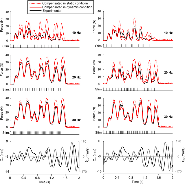
Figure 6. Force production during dynamic variations in length and frequency in CT95. Force responses of the actual muscle (CT96), the model compensated under the static (equation (18)) and dynamic condition (equation (20)) were compared with constant (right column) and random (left column) excitation frequencies (10, 20, and 30 Hz) under the same random variations in length (Xm) between 0 and −16 mm. The rate ( of length change is indicated as a solid gray line at the bottom panel. The model parameter values set for CT95 were fully presented in table 1.
Download figure:
Standard image High-resolution image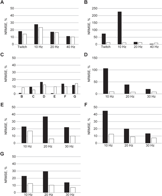
Figure 7. NRMSE (%) between the actual and model muscle. (A), (B) NRMSEs for the default (black filled bar) and compensated model (empty bar) in figures 2(A), (C). (C) NRMSEs for the inverse (black filled bar) and new model (empty bar) in figure 3(B)–(G) in the abscissa correspond to figures 3(B)–(G)). (D), (E) NMRSEs for the model compensated under static (black filled bar) and dynamic (empty bar) condition in figures 4 and 5. (F), (G) NMRSEs for the model compensated under static (black filled bar) and dynamic (empty bar) condition in the left and right column of figure 6. Note the different scale in each panel.
Download figure:
Standard image High-resolution image
4. Discussion
Here, we have investigated the dependencies of the muscle activation dynamics (A(t)) on excitation and movement, and proposed the modified Hill-type muscle model that reproduces force production from the soleus muscles for the static and dynamic variation in two input signals (excitation frequency and muscle length). While comparing the model with actual muscles, we observed a strong dependency of A(t) on muscle length during static (i.e., isometric) contractions. As the length was varied dynamically, the suppression of A(t) over lengths below the optimal length together with movement-induced activation degradation at low frequencies were crucial for the prediction accuracy of the proposed model. These results emphasize the importance of considering the influence of length and frequency on muscle activation to accurately simulate Hill-type muscle models under static and dynamic conditions.
4.1. Comparison with previous studies
In the previous studies, the dynamics of muscle activation has been investigated under limited conditions in excitation frequency and muscle length. The dependence of A(t) on the frequency and the length has been evaluated and modeled for static (i.e., isometric and isokinetic) contractions at various frequencies (Brown et al 1996, Hatze 1977, Wexler et al 1997, Brown et al 1999, El Makssoud et al 2011). In other hand, the movement dependency of A(t) has been characterized and formulated under tetanic or tetanic-like excitation (Shue and Crago 1998, Williams et al 1998). In the present study, we have evaluated and identified the frequency and length dependencies of A(t) while systematically varying the frequency (twitch to tetanic) and the length (isometric to locomotor-like movement) over the full physiological range. What we have found critical from the present analysis is that the phenomenon of movement-induced activation degradation at the low frequencies should be taken into account for realistic modeling of A(t) during movement (figure S3).
A modular framework has been applied to model the activation dynamics based on three signal transductions (i.e., neural excitation → [CaSP] → A(t) → muscle force) during force production (Wexler et al 1997, Williams et al 1998, El Makssoud et al 2011, Laforet et al 2011). In previous modeling approaches, all model parameters have been optimized to match the overall input–output properties of target muscles under limited conditions, such as isometric contractions, sinusoidal movement or full excitation. The simultaneous adjustment of all model parameters may give rise to several numerical issues related to optimization time, parameter redundancy, and stability because the number of parameters typically increases with increases in the complexity of input conditions and muscle responses. To avoid these issues while increasing computational tractability, we have determined the model parameter values separately for individual modules directly based on relevant data.
The muscle models have been implemented in the software environment that is not in favor of building and simulating realistic motor neuron models. In the present study, the features of our modular modeling approach proved to be useful for the implementation in NEURON software environment, which supports compartmental modeling, addition of new biophysical mechanisms, and independent manipulation of inserted mechanisms for multi-purpose simulations. To our knowledge, this is the first demonstration for the possibility of incorporating mechanical mechanisms into NEURON platform. Our muscle modeling approach implementable in general neuron simulators will be particularly convenient for studies coupling output of models of spinal motoneurons (e.g., (Carlin et al 2000, Elbasiouny et al 2006, Kim et al 2014)) to muscle fibers.
The transduction of [CaSP] to A(t) has been captured by modeling the chemical reactions between actin and myosin molecules in either a simplified (Wexler et al 1997, Williams et al 1998) or detailed form (Laforet et al 2011). In previous studies, all model parameters were simultaneously optimized to fit the overall input–output properties. Thus, it has been uncertain whether previous models could capture the cooperative effects of Ca on force production that have been characterized by the nonlinear (i.e., logistic) relationship between [CaSP] and force in both computational (Shames et al 1996) and experimental (Backx et al 1995) studies. In this study, the [CaSP]-force relationship was dynamically represented in Module ② using the Morris–Lecar formulation, and its five parameters (C1–C5 in equation (8)) were adjusted to match the twitch and sub-tetani of actual muscle at an optimal length. As a result, the sigmoid shape of the [CaSP]-to-force relationship in the steady state (see the  –[CaSPT] curve in Module ②, figure 1) and the slow kinetics of the activation dynamics (see
  in Module ②, figure 1) in our model were consistent with those reported in previous studies. In addition, the
  did not significantly vary over a wide range of [CaSPT], suggesting that the dynamics of the [CaSP]-to-force transduction might be described with only two parameters (C1 and C2) for the
  -[CaSPT] relationship under the assumption of a constant time constant. Furthermore, to determine whether the nonlinear shape of the [CaSP]-to-force relationship was important, we compared this case with the linear relationship of the [CaSP] to force. The comparison results indicated that the model with a linear relationship resulted in significant simulation errors during the sub-tetanic responses of the cat soleus muscle over a physiologically relevant frequency range (figure S2). These results indicate that the nonlinear relationship between the [CaSP] and force should be reflected in accurate simulations of muscle responses for a wide range of input conditions.
In the present study, the dependencies of A(t) were investigated for slow (i.e. soleus) muscles of cats. During isometric contractions, the amplitude of A(t) was more sensitive to the shortening relative to the lengthening (figures 2(D)–(F)). In addition, the length dependency of A(t) was prominent at low rather than high level of excitation frequency (figures 2(A)–(C)). These findings are similar to those reported in the previous studies for fast (i.e. caudofemoralis) muscles of cats (Brown et al 1999). This result suggests that the length and frequency dependency of A(t) in isometric conditions seem to be a generic feature, not type specific.
For tetanic muscle behavior, the post-activation potentiation (PAP) after activities has been experimentally shown in fast muscles of cats and reported to make rise and fall times of tetanic response faster and slower respectively when potentiated (Brown et al 1999). In the present study, the potentiated (or slow) force relaxation following excitation was found in one (i.e. CT09) of slow muscles for twitch and sub-tetanic contractions when compared to the model not considering the PAP phenomenon (figures 2(A) and (B)). However, this result was not obvious in the other muscle preparation (i.e. CT95) (see figure S1). Thus, further works would be needed to clarify if and how the PAP affects force production of slow muscles.
The length dependency of contractile activation has been shown to be related to the decrease in the contractile protein sensitivity to Ca2+ at shortened lengths, leading to degradation of the activation level (Stephenson and Wendt 1984). As predicted from this experimental observation, the default model without length-dependent compensations significantly overestimated activation dynamics when the length was shortened below the optimal length (see figure 2(F)). This shortening-induced activation degradation was reflected by making a single rate constant (K5 in figure 1) for the Ca2+–troponin reaction as a function of length. As a result, the compensated model with K5 modulated according to the length change matched the rising phase of the force development well during twitch and sub-tetanic contractions. However, this compensation via K5 modulation was not sufficient to reproduce the potentiated (or slow) relaxation dynamics of muscles after the end of excitation (figures 2(A) and (B)). This result suggests that other factors inducing the force enhancement, such as nonlinear Ca2+ dynamics in SP (Otazu et al 2001, Cheng et al 2013), passive filament components (e.g., titin,(Nishikawa et al 2012)) or active molecular modulation (e.g., phosphorylation of myosin regulatory light chain, (Sweeney et al 1993)), are likely to be involved during the relaxation phase of muscle contraction in soleus muscles.
Error in the Hill-type muscle model has been reported to be prominent during muscle movement (Sandercock and Heckman 1997b, Perreault et al 2003, Millard et al 2013). In the present study, we further demonstrated that model error could also be significant at physiologically relevant frequencies even during isometric contractions (figure 2(E)). The error found between the model and actual muscle during movement was attributed in part to the hyperactivation of the models at lengths shorter than the optimal length (figure 4), which is similar to the results obtained for isometric contractions (figure 2). The model error associated with hyperactivation during movement was compensated for based on the formulation consisting of muscle length and velocity, as suggested for a slow change in muscle length and wide width of pulse stimulation in the previous study (Shue and Crago 1998). In our case, in which the muscle moved in a relatively fast mode with impulse excitation, the dependence of the activation dynamics on length and velocity was found to be dominant for lengths less than the optimal length during the positive velocity movement (gray areas in figure 4). As a result, the mechanism compensating for this A(t) dependency was effective to reduce the model error particularly for the phase of force development during locomotor-like movement.
The movement-induced force depression (Gillard et al 2000) was relatively more significant during movement under low frequencies (≤20 Hz in figure 4, see also the top panel in figure S3). This force depression phenomenon appears to not be related to fatigue-like effects but to the activation degradation induced by the movement in soleus muscles. Because the molecular mechanisms underlying this movement-induced force depression remain unclear, we compensated for this model error by gradually increasing α in Module ② to give rise to a slow reduction in the activation level during movement (figure S3). However, the similar movement induced effect on force depression was also possibly obtained by changing other factors including K1, K2, Rmax, K5 and K6i from their initial values. Thus, the systematic sensitivity analysis for the default model parameters might allow the investigation of potential biophysical mechanisms underlying the movement-induced force depression. All of these results support that the movement-induced activation degradation is prominent factors influencing the activation dynamics of cat soleus muscles during movement.
Direct comparison of the compensation mechanisms for dependencies in the activation dynamics between this and previous studies is difficult due to differences in the input conditions, force mechanism (Huxley versus. Hill-type) and species in which individual studies have been interested. In this study, we focused on force production in adult cat soleus muscles over a wide range of input conditions for excitation frequency (1–100 Hz) and length change (e.g., isometric, isokinetic, and dynamic). Furthermore, this study is the first to demonstrate the applicability of Hill-type models for a full physiological range of excitation frequency and muscle length in mammals. The Hill-type muscle model has been ubiquitously employed in many large-scale simulations mainly for the bio-mechanical analysis of motor performance in human and animals (Biewener et al 2014). Our modified Hill-type muscle model would make significant contribution to not only improving the reliability of musculoskeletal simulations of movement, but also extending the usage of these simulations to the study of neural mechanisms underlying movement control.
4.2. Limitations of the current model for activation dynamics
There are several muscle behavior properties that the current model does not consider, most likely due to our lack of knowledge of the underlying molecular mechanisms. Firstly, the new Hill-type model may not produce a post-excitation force depression for shortening (figure 3(D)) and post-excitation force potentiation for lengthening (figure 3(F)) during isometric contractions following isokinetic contractions under full excitation (De Ruiter et al 1998, McGowan et al 2010). The underlying mechanisms of this velocity dependent force redevelopment remain unclear (Shue and Crago 1998), although several possibilities have been recently suggested, including the length-dependent change in the Ca2+ sensitivity of myofilaments (Fuchs and Martyn 2005) and the winding filament theory which emphasizes the role of the elastic protein titin in force production at different lengths (Monroy et al 2012, Nishikawa et al 2012).
Secondly, the current model may not generate nonlinear force development in response to initial multiple impulses with short intervals (i.e., 5–10 ms) (known as duplet potentiation, (Sandercock and Heckman 1997a)). For random stimulation frequency with the mean of 10 Hz, the actual force was almost three times larger than the model prediction after multiple impulses with 13 ms inter-stimulus interval, indicating force potentiation probably induced by the doublet effect (see top panel in figure 5).
Thirdly, the variability in the degree of A(t) dependency on the static and dynamic contractions was found in two soleus muscles (CT09 ad CT95) used in this study. Due to the small sample size, however, it is inconclusive whether and how the A(t) dependency degree is different for the population of soleus muscles. For clarification of this issue, further investigation would be needed with a sample size with sufficient statistical power.
Fourthly, we have developed a new Hill-type muscle model based on data measured from cat soleus muscles. The soleus muscles have been known to consist mainly of the slow type of muscle fibers (McPhedran et al 1965b, Ariano et al 1973). Thus, the type specificity of the compensation mechanisms built in this model should be further tested for the muscles that contain the fast type of muscle fibers or a mixture of slow and fast muscle fibers (McPhedran et al 1965a, Ariano et al 1973). In addition, further works would also be needed to evaluate the generality of the new modeling approach across animals.
Finally, the new muscle model developed in this study may have a potential to be used for a building block in physiologically reconstructing and simulating a population of motor units (a motoneuron and muscle fibers that it innervates). However, the experimental data used to determine the model parameters were collected while applying the electrical spikes and length change to the whole soleus muscle. Even though the data might represent the average input–output properties of S-type muscle fibers, in order to link directly with motoneuron models for biological realism the model parameter values derived from this study should be further evaluated against the data obtained in the level of single motor units.
4.3. Conclusions
Hill-type formulation of muscle dynamics is a powerful tool for large-scale simulations due to its simplicity and intuitivism. In this study, we have extended the applicability of the Hill-type modeling approach by developing a model of activation dynamics that allows for not only muscle simulations under physiologically relevant excitation and movement but also computationally efficient implementation in neuron simulators in which neuron models are generally reconstructed. We hope that the modified Hill-type modeling approach enhances the accuracy of neuro-musculo-skeletal simulations and thereby contributes to advancing our understanding of the neural mechanisms underlying movement control.
Acknowledgments
This work was supported by National Institutes of Health Grant R01 NS071951 and NS062200, and the DGIST R&D Program of the Ministry of Science, ICT and Future Planning of Korea (13-01-HRSS-03 and 14-RS-02).