
Abstract
Objective: Subjective tinnitus is an auditory phantom perceptual disorder without an objective biomarker. Fast and efficient diagnostic tools will advance clinical practice by detecting or confirming the condition, tracking change in severity, and monitoring treatment response. Motivated by evidence of subtle anatomical, morphological, or functional information in magnetic resonance images of the brain, we examine data-driven machine learning methods for joint tinnitus classification (tinnitus or no tinnitus) and tinnitus severity prediction. Approach: We propose a deep multi-task multimodal framework for tinnitus classification and severity prediction using structural MRI (sMRI) data. To leverage complementary information multimodal neuroimaging data, we integrate two modalities of three-dimensional sMRI—T1 weighted (T1w) and T2 weighted (T2w) images. To explore the key components in the MR images that drove task performance, we segment both T1w and T2w images into three different components—cerebrospinal fluid, grey matter and white matter, and evaluate performance of each segmented image. Main results: Results demonstrate that our multimodal framework capitalizes on the information across both modalities (T1w and T2w) for the joint task of tinnitus classification and severity prediction. Significance: Our model outperforms existing learning-based and conventional methods in terms of accuracy, sensitivity, specificity, and negative predictive value.
Export citation and abstract BibTeX RIS

Original content from this work may be used under the terms of the Creative Commons Attribution 4.0 license. Any further distribution of this work must maintain attribution to the author(s) and the title of the work, journal citation and DOI.
1. Introduction
Subjective tinnitus is an auditory phantom disorder characterized by the perception of internally generated elemental sounds, often described as ringing, humming, buzzing, chirping, or clicking, in the absence of externally identifiable sources. In its chronic phase, tinnitus manifests as a central nervous system disorder. Some prevailing hypotheses include maladaptive neuroplasticity, misappropriated attention, and dysfunctional striatal gating [1–3]. While often accompanied by hearing loss, tinnitus severity or distress is often modulated by comorbid anxiety, depression, or mood disturbance. Bothersome tinnitus can degrade activities of daily life, disrupt sleep, and decrease work productivity [4]. There is a need for the scientific community to develop novel diagnostic methods to advance tinnitus management along its entire clinical course—starting from detecting or confirming the condition, progressing to tracking change in severity, and concluding in monitoring treatment response. This challenge in clinical tool development may be approached by machine learning methods [5] that categorize a patient into binary or multiple classes for tinnitus presence and regression models of continuous clinical assessment values for estimating tinnitus severity.
Neuroanatomical and neurophysiological evidence point to tinnitus-related reshaping of the auditory pathway, with subtle reorganization of auditory areas (cortical and sub-cortical) over time, and widespread structural and functional changes across the whole brain (WB) [6–9]. Various neuroimaging techniques have been used to demonstrate structural abnormalities in the brain of tinnitus patients. White matter (WM) tracking using diffusion tensor imaging shows alterations in both auditory and limbic areas [10]. Grey matter volume (GMV) extracted from structural MRI (sMRI) shows significant changes in various areas of tinnitus patients compared to healthy controls [11, 12]. A decline in GMV has also been reported in ventromedial and dorsomedial prefrontal cortices, nucleus accumbens, anterior and posterior cingulate cortices, hippocampus and supramarginal gyrus [12–14]. In our own recent work, we have shown evidence for volumetric changes within auditory and limbic networks in tinnitus subjects [15]. Specifically, we have shown that the volume of corpus callosum and other structures are altered in tinnitus patients using a priori brain regions as manually selected features. The current study builds upon neuroanatomical alterations in tinnitus with the objective to discover predictive anatomical features for tinnitus classification. It is possible that in addition to subtle volume changes, there may also be shape or texture changes in brain images that are important for tinnitus classification. It is also not clear whether volume changes alone would have predictive value for tinnitus classification. There is a need to move beyond manually selected features that include shape and texture in an automated process.
Here, we take an automated approach with deep neural networks that subsumes and advances previous investigations of neuroanatomical changes associated with tinnitus. By examining the raw brain images directly, the automated features selected include shape, texture and microstructural integrity as well as volumetric changes. Deep neural networks are ideally suited to automatically extract relevant features embedded in brain images, and therefore are expected to be more sensitive for tinnitus classification. In turn, this effort would enable more robust development of mechanistic structure-function models of tinnitus in the future. Therefore, in the current study, our focus is to develop a data-driven framework for simultaneous tinnitus classification: presence or absence of auditory phantom percepts, and estimation of tinnitus severity. Specifically, we aim to apply statistical and machine learning algorithms to sMRI data for the following objectives: (1) assess sMRI-based algorithm performance to differentiate tinnitus patients from healthy controls, and (2) identify the key sMRI features most strongly associated with clinical rating of tinnitus severity.
1.1. Related work
In this section, we briefly review prior work on neuroimaging-based methods for diagnosis of several neurological diseases and tinnitus. A critical consideration for optimizing clinical tool performance is choice of feature space for neuroimaging data extraction [16–18]. In terms of MRI feature representations, there are three categories: (1) voxel-based features [16] such as WM, grey matter (GM), and cerebrospinal fluid (CSF), (2) region-of-interest (ROI) based features [17] including regional cortical thickness, hippocampal volume, and GM volume, and (3) patch-based features [18]. Amongst these feature classes, voxel-based features possess higher degrees of freedom—millions of voxels. These are independent of any hypothesis of brain structures. However, dimensionality reduction of the high dimensional data remains an integral part of voxel-based disease prognosis. Inspired by the tremendous success of deep learning [17], we choose automated image feature extraction over a hand-crafted feature approach.
Many researchers have made promising contributions using deep learning methods for classification and regression models for symptom prediction in a variety of brain disorders, including Alzheimer's disease (AD) [19–23], dementia [24, 25], and autism [19, 26–28] but none exists for tinnitus. Zhou et al introduced a multimodal approach by integrating MRI and positron emission tomography for early dementia diagnosis [29]. A graph convolutional neural network (CNN) that leverages both imaging and non-imaging information for brain analysis in large populations with autism disorder has been performed [19]. Graph nodes are associated with imaging-based (functional MRI) feature vectors within the classification framework in data obtained from patients with autism and AD. A deep learning framework to classify AD based on WB sMRI using hierarchical structure of both voxel-level and region-level features has been proposed [20]. Yet another deep learning method based on sMRI has been introduced [21] to jointly detect AD disease and predict clinical scores. Oh et al [23] proposed a sMRI volumetric CNN using an end-to-end learning approach for AD classification and spatial attention visualization. Neuroimaging with computer-aided algorithms have made remarkable advances in dementia prognosis [24]. In particular, Xia et al [25] proposed a novel dementia recognition framework based on deep belief network using functional MRI. Arya et al [26] developed a graph convolutional network by fusing structural and functional MRIs for autism classification. Understanding the structural components of human brain that capture discriminating features for various brain disorders is of broad interest to computational neuroscience [30]. In particular, recent work on mild cognitive impairment classification [31] identified ROI with substantial influence on the classification task. We note that the study on correlation between GM and WM degeneration in various brain disorders is a potential experimental research direction [32–35]. Recent experimental findings suggest that tinnitus could potentially reorganize anatomical substrates in the brain [15, 36, 37]. Motivated by these studies, we consider exploring how these anatomical substrates (GM, WM, and CSF) could impact to our method.
We note that limited efforts using analytical and deep learning frameworks have been made for tinnitus detection and tinnitus severity prediction. Shoushtarian et al [38] investigated the sensitivity of functional near-infrared spectroscopy (fNIRS) to differentiate individuals with and without tinnitus and to identify fNIRS features associated with subjective ratings of tinnitus severity. A machine learning method, including feature extraction and classification were applied to fNIRS data. An analytical approach based on whole-brain functional connectivity and network analysis was introduced for binary tinnitus classification [39]. A combined dynamic causal modeling and exponential ranking algorithm applied to EEG data yielded new insights into abnormal brain regions associated with tinnitus [40]. An unsupervised learning framework using a spiking neural network to analyze EEG data captured neural dynamic changes [41], extending earlier EEG based classification methods [21]. To the best of our knowledge, this is the first effort to explore deep learning for joint tinnitus classification and tinnitus severity prediction using sMRI data.
1.1.1. Deep multi-tasking in medical image analysis
Multi-tasking networks are of special interest to the deep learning research community, where common discriminator features across multiple tasks could be learned from input data [21, 42–47] including multimodal medical imaging data [48]. For instance, multi-tasking networks in [42] combined models for regression and classification of lung nodules used in CT images. Stacking computational features derived from a deep learning auto-encoder and a CNN resulted in superior performance when compared to single task networks [42]. Similarly, authors in [46] introduced a novel multi-tasking deep framework for both regression and classification of AD to successfully identify AD-relevant biomarkers. Multi-tasking reconstruction and segmentation of brain MR images was also successfully reported in [47] with impressive performance. Inspired by [47], here, we introduce a novel deep network framework for jointly solving classification models for tinnitus diagnosis and regression models for tinnitus severity prediction.
1.2. Scientific contributions
The main contributions are:
- (a)Multi-tasking deep analysis for classifying tinnitus presence and predicting tinnitus severity: We propose a CNN built on a ResNet architecture for multi-tasking analysis of tinnitus using sMRI with WB 3D voxel-level features for jointly performing tinnitus classification and tinnitus severity prediction.
- (b)Multimodal fusion and Structural Controllability: We combine features from both T1-weighted (T1w) and T2- weighted (T2w) sMRI within our network. Integration of multimodal structural imaging data within a joint framework leverages the strength of each modality and their inter-relationships for multi-tasking performance. Furthermore, we determine imaging features (WM, GM, CSF) that contribute to tinnitus classification and tinnitus severity prediction performance by examining them individually and collectively.
- (c)Multi-tasking loss function: We introduce a novel loss function for efficient learning in multi-tasking network. In particular, the proposed loss function jointly penalizes both classification and prediction performance by convex combination of the individual losses. To mitigate shortcomings of class imbalance, we use a focal loss [49] function. We also use data augmentation to avoid over-fitting during training.
- (d)Evaluation of clinical tool performance using the largest tinnitus dataset: We validate our proposed framework on the largest tinnitus datasets available to us from collaborative research between the University of California, San Francisco and the University of Minnesota. With elaborate experiments, we show that our method achieves superior classification accuracy over state-of-the-art approaches while simultaneously predicting tinnitus severity scores from multimodal sMRI data.
1.3. Organization
In section 2, we describe the dataset in detail and explicate the data processing pipeline. In section 3, we explain our proposed deep learning method: fundamental architecture, fusion of sMRI T1w and T2w images, and dual-tasking framework. In section 4, we present experimental results comprehensively and compare our method against the support vector machine (SVM) benchmark. In section 5, we discuss our experimental finding and the connection and relevance of our work to state-of-the-art methods for tinnitus. In section 6, we provide concluding comments.
2. Methods
In this section, we introduce the sMRI datasets used in our analysis. We further discuss the details on data collection and preprocessing steps.
2.1. Dataset
MRI data from 379 total subjects were used as the training dataset from two recruitment sites—University of California San Francisco (UCSF) and University of Minnesota. Both T1-weighted (MPRAGE) and T2-weighted images were acquired at both sites using standardized parameters according to the Human Connectome Project optimized for each machine, making them comparable across sites [50]. At UCSF, a GE MR750 3.0 T machine was used to acquire both T1w (226 0.8 mm slices, in-plane resolution: 0.8 mm × 0.8 mm, flip angle = 8 degrees, TE = 2 ms, IT = 1060) and T2w (208 1 mm slices, in-plane resolution: 1 × 1 mm, flip angle = 90 degrees, TR = 3200 ms, TE = 67 ms) scans. At University of Minnesota, a Siemens MAGNETOM Prisma 3.0 T machine was used to acquire both T1w (208 0.8 mm slices, in-plane resolution: 0.8 × 0.8 mm, flip angle = 8 degrees, TE = 2 ms, IT = 1000 ms) and T2w (208 0.8 mm slices, in-plane resolution: 0.8 mm × 0.8 mm, flip angle = 120 degrees, TR = 3200 ms,TE = 563 ms) scans. In total there were 183 tinnitus patients and 196 normal controls (table 1, top and middle rows show the site distributions). All these subjects are used for As 44 UCSF subjects underwent two data acquisition sessions, data from the first or second session was chosen for use as the independent validation dataset (table 1, bottom row). Tinnitus or control binary labels and their corresponding structural images were fed into the model for the classification task. Further, there were 240 subjects from the training dataset that also completed the Tinnitus Functional Index (TFI) [51], which measures tinnitus on a continuous scale from 0 to 100. Data from those subjects were fed into the regression model. There were 24 subjects from the independent validation dataset with TFI scores that were used for further model evaluation.
Table 1. Demographic and clinical information of the training/validation and independent dataset.
| Tinnitus | Control | ||
|---|---|---|---|
| UCSF | Number of subjects | 95 | 84 |
| Female/male | 33/62 | 41/43 | |
| Age (mean ± SEM) | 56.4 ± 13.6 | 44.3 ± 18.0 | |
| Univ. of Minnesota | Number of subjects | 88 | 112 |
| Female/male | 39/49 | 64/48 | |
| Age (mean ± SEM) | 50.5 ± 15.2 | 34.5 ± 13.8 | |
| Independent Validation Dataset (UCSF) | Number of subjects | 24 | 20 |
| Female/male | 6/18 | 10/10 | |
| Age (mean ± SEM) | 57.3 ± 14.3 | 42.8 ± 19.1 |
2.2. Data processing
All T1w and T2w sMRI images are subjected to the same processing steps for quality control and image alignment. The clinical MRI scans contain irrelevant bony skull, soft tissue, and cervical regions, and variations in spatial orientation of acquired images that may affect clinical tool performance. Images were coregistered and aligned to template space (FSL toolbox, [52]) via a standard mask generation method [53] in three steps. First, structural images are processed with a skull-strip step that removes the skull and other soft tissue regions that are outside of the cortex. Second, skull-stripped images are registered into a MNI-152 2 mm template space that aligns the structural data spatially. Finally, registered image data are processed with the intensity normalization step. These operations remove artifacts due to magnetic field inhomogeneity from different MRI scanners. The pre-processed data are treated as the 3D volumetric input of the classification and regression task.
To identify and compare features of the volumetric whole-brain images and segmentations that drive performance, regions corresponding to CSF, GM and WM are generated (FSL toolbox, [52, 53]) and segmented [54] for T1w and T2w images used in both classification and regression tasks. An example of the brain tissue segmentation process [54] is shown in figure 1. Skull-stripped images that exclude soft tissue regions not considered within the brain cavity were submitted to segmentation based on a hidden Markov random field model and optimized via expectation-maximization algorithms [53]. This pipeline considers spatial information in terms of mutual information available in local neighborhoods, and includes corrections for spatial intensity variations to overcome the bias field to classify voxels into WM, GM, and CSF.

Figure 1. The workflow of brain segmentation process with FSL toolbox [53] to generate CSF, GM and WM segmentations.
Download figure:
Standard image High-resolution image3. Algorithm
We start this section with the architecture of our proposed multi-tasking algorithm. This is followed by a novel loss function to train the network for multi-tasking. Subsequently, we discuss the implementation details including data augmentation and transfer learning. The performance metrics to evaluate the performance of classification and TFI score prediction are also described. We also provide brief details of benchmark comparison algorithms which are compared later.
3.1. Proposed architecture
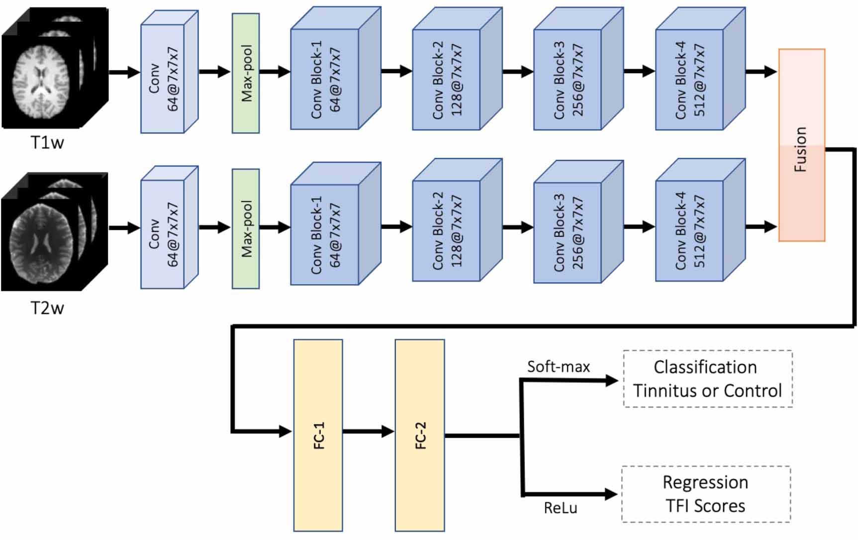
The algorithm for joint classification and regression tasks for tinnitus is built on ResNet-18 deep neural network architecture [45], which includes the residual information extracted from the previous layer and mitigates the adverse performance by using large number of layers. We used a significantly modified ResNet-18 architecture as our backbone that incorporates both multiple modalities of imaging and the multi-tasking goals of our network. One attractive aspect of our method is the efficient integration of both modalities processing sMRI data from each subject. In particular, the network consists of two parallel feature extraction sub-networks: one for T1w and another for T2w. The outputs from both sub-networks are concatenated. The fused composite features are further processed for joint tasking as shown in figure 2. Each of the sub-networks consists of 17 convolutional layers. The first convolutional layer takes the input and applies filters for the following convolutional layer input. Sixteen convolutional layers are wrapped into four convolutional blocks with four layers in each block. Note that same number of convolutional filters are used in each of convolutional blocks. For example, there are 64 filters in each convolutional layer of the first convolutional block. Each convolutional layer (within each convolutional block) follows with a batch normalization and a ReLu layer for more efficient gradient convergence (i.e. accelerate the training process) and only allows the positive values to pass to the next layer. Further, after each convolutional block, extracted features are pooled. The output from the fourth convolutional block of the two sub-networks are the features extracted from T1w and T2w data separately. We flatten each feature map into 1D array to combine features. Next, we concatenate two 1D arrays into a longer length of feature array. This simple fusion step essentially creates a double length fused feature array. The extended feature array is passed through two fully connected layers with different dimensions. The output layer of the final fully connected layer FC-2 in figure 2 is used for multi-tasking: to simultaneously predict the class probability (via soft-max) and estimate the TFI score. The proposed deep learning method is referred to as multimodal multi-tasking convolutional network (MMCN).

Figure 2. Overview of the proposed multimodal multi-tasking convolutional network (MMCN) for joint classification and regression of tinnitus. The pipeline takes the volumetric sMRI for both T1w and T2w as input in the first convolutional layer. There are four convolutional blocks in each sub-network. In each block, there are four convolutional layers that take the learned features from the previous block. Each convolutional layer in the block is followed by a batch normalization and a ReLu layer to converge the gradient more efficiently and accelerate the training process. A pooling layer is applied at the end of each convolutional block to down sample and retain useful features. The filter sizes of each convolutional block are 64, 128, 256 and 512, respectively. A fusion step is applied after the final convolutional block to concatenate the features from each of the sub-networks. Further, two fully connected layers are used to learn non-linear combinations from the feature map. In the output layer, soft-max is used for tinnitus classification and ReLu is adapted for the regression task tinnitus severity prediction based on TFI scores.
Download figure:
Standard image High-resolution image3.2. Proposed multi-tasking loss function
3.2.1. Loss function for classification
We examined two different loss functions for optimization of the classification performance, specifically, cross-entropy and focal loss [49]. Let the training set consisting of N number of subjects defined as  . Each subject has a label
  which indicates whether the subject is a healthy control or a tinnitus patient. The cross-entropy loss for binary classification is defined as follows:

where  is an indicator function; W is the collection of learned network coefficients and
  indicates the probability of subject Xn
being correctly classified as the correct label
indicates the probability of subject Xn
being correctly classified as the correct label  . Note that
  if the condition
  is true and 0 otherwise.
The labels of classification task in our setting are either tinnitus patient or healthy control. However, an imbalanced dataset may lead to suboptimal training of the network. To deal with the limitation of class imbalance in the dataset, we instead use focal loss [49], which is a modified version of the commonly used cross-entropy. Focal loss uses a modulating factor on top of the original cross-entropy equation, with tunable focusing parameter  . It is denoted as follows:

where  . We empirically choose λ = 2. In fact, we experiment with different values of λ. Finally, we find λ = 2 to produce the most consistent results.
3.2.2. Loss function for regression task
To guide the training of the regression task, we minimize L2 distance between the predicted and actual TFI scores. Suppose, there are K numbers of discrete TFI scores in our dataset such that  . The mean squared loss between the estimated TFI score and the ground truth is

where  is the predicted TFI score of subject n.
3.2.3. Loss function for multi-tasking
The training operation in the multi-task network is controlled by a loss function which could jointly penalize the error of both classification and regression tasks. In fact, we consider a convex combination of the cross-entry (or focal) and L2 loss. In particular, we use the following two composite losses:

where ![$\alpha \in [0, 1]$](https://content.cld.iop.org/journals/1741-2552/20/1/016017/revision3/jneacab33ieqn12.gif) is a coefficient tuned using cross-validation. The convex combination controlled by α leverages an improved joint learning. The optimal value of α is set using cross-validation. We note that α may vary depending on class imbalance and distribution of the ground truth TFI scores in the datasets used. However, the protocol of setting α using cross-validation ensures the best possible training of the deep network.
is a coefficient tuned using cross-validation. The convex combination controlled by α leverages an improved joint learning. The optimal value of α is set using cross-validation. We note that α may vary depending on class imbalance and distribution of the ground truth TFI scores in the datasets used. However, the protocol of setting α using cross-validation ensures the best possible training of the deep network.
3.3. Implementation details
The implementation of the proposed CNN model is based on the Pytorch library. The experiments are conducted on a NVIDIA GTX TITAN 16 GB GPU. We optimize the learning rate, and find the optimal value to be 10−4. We use stochastic gradient descent (SGD) approach for optimization [55]. The network gradients while performing optimization are combined with the back-propagation algorithm. The learning rate for SGD are empirically set to 10−3.
We adopt the transfer learning to overcome the challenges with limited number of subjects. Transfer learning is widely used for obtaining the weights for problems in the same domain to reduce the training time, to improve the overall performance, and to decrease over-fitting. Here, we use pre-trained parameters from MedicalNet [56] as weights for all four convolutional blocks. Therefore, we only learn the weights of the subsequent portions of the network. We follow the same form of transfer learning for both classification and regression prediction tasks. In summary, our proposed MMCN network learns the fully connected layers with transfer learning applied to the convolutional weights.
3.4. Data augmentation
Availability of sufficient amount of data for adequately training a deep network is often a real concern in medical imaging. In fact, it is recommended to have at least 1000 samples of each class to train a classification model. To overcome the limitation of this high data requirement, we performed data augmentation which also helps to avoid data over-fitting during the training. The goal of evaluating classification performance using an independent dataset is to validate the robustness of training.
Data augmentation is a process to create new artificial data by altering the available data set. It has by many been considered a key factor for increasing robustness and performance of image classification tasks using deep learning methods, such as the CNN. Our method consists of three kinds of elementary operations—random flip, random affine transform and random elastic deformation. The only nonlinear transformation within our data augmentation is elastic transformation, which is basically used to simulate motion artifacts in MR images [57]. We note the article that presents U-Net [58] claims that it was a particularly important augmentation for MR images.
We perform on-the-fly data augmentation using two strategies, i.e. (i) randomly flipping the sMRI for each subject, and (ii) randomly distorting the sMRI with non-linear transformation for each subject. The operation of random shifts introduce a reasonable perturbation to the training data to learn the useful features. When combined with the first two operations, it could effectively augment the number and variability of available samples for training our MMCN model.
3.5. Performance metrics
We examine the effectiveness of the proposed framework for the multimodal multi-task learning-based test data and the independent dataset. To prevent the introduction of potential bias for not including the entire dataset, we construct non-overlapping five-fold cross validation in the training process. Specifically, we randomly select 20% of the sample size from each class as the testing dataset, while the remaining 80% of the subjects are treated as the training dataset. This way we successfully utilize the existing available subjects to produce an unbiased performance.
Classification performance is evaluated by five metrics, including classification accuracy (ACC), sensitivity (SENS), specificity (SPEC), positive predictive values (PPV), and negative predictive values (NPV). These standard metrics are defined as [20]:

where TP, TN, FP, and FN denote the true positive, true negative, false positive, and false negative values respectively. For all these five metrics, a higher value indicates a better classification performance.
Regression performance is measured using an r-squared (r2) metric, which is a statistical measure that represents the proportion of the variance for a dependent variable that's explained by an independent variable or variables in a regression model [59]. The definition of the coefficient of determination is as follows. Suppose the ground-truth and predicted TFI scores of nth subject are given by qn
and  . There are total N subjects used for testing to evaluate the regression performance. Also, we refer the mean of the ground-truth scores of all subjects as
  . Then, the r-squared (r2) metric is defined as:

We clearly see from the above expression in (2) that it will take values between 0 and 1. At perfect prediction of TFI scores, by setting  for all n in (2), we obtain
  . In summary, a higher value of r2 indicates a better regression performance achieved by the proposed method.
3.6. Influence of brain tissues on multi-tasking
We perform an additional investigation to understand whether the WB MRI or a particular brain tissue (CSF, WM, or GM) plays a dominant role in the multimodal multi-tasking performance of our method. In particular, both T1w and T2w images are first segmented into respective GM, WM, and CSF components [54]. Thus, including WB, we get total four sets of data for each subject. The detailed steps of using WB data into our network are explained in figure 2. For the analysis using these three structural segments, we simply substitute the respective segment of both T1w and T2w images. For example, to perform the joint tasking based on GM, we use GMs derived from T1w and T2w respectively as inputs. We follow similar steps for both WM and CSF based joint tasking. Note that we perform the training and test for these four cases (WB, CSF, GM, and WM) completely independently. This independent way of training the network (for each of those four sets of input) allows to one to learn a joint multi-tasking selection parameter α in (1) in the best possible way.
3.7. Benchmark methods
Our MMCN method is first compared against two conventional learning-based methods—least squares support vector machine (LS-SVM) [60] and K-nearest neighbor (KNN) [61]. In addition, MMCN is compared with a state-of-the-art deep-learning method, hierarchical fully convolutional network (H-FCN) [20], which has been used to extract useful features from imaging data to classify AD as we are unaware of a similar method for tinnitus classification or severity prediction. We now briefly summarize the three benchmark methods.
- (a)LS-SVM: We use a modified version of SVM, a widely used classification model in neuroimaging analysis [60, 62]. We directly train a least squares SVM model on T1w WB volumetric MRI images that contain all available structural information. The trained model is applied on the test data to obtain final classification results in the test sample.
- (b)KNN: K-nearest neighbor is another popular classical method used for performing unsupervised classification. This simple machine learning algorithm is based on the distance between feature vectors [61]. The KNN algorithm classifies new unknown data points by finding the most common class among the k-closest centroids. In our case, T1w WB volumetric MRI of each subject is treated as sample points for KNN algorithm. Test subjects are classified based on neighborhood of the learned centers (k-means).
- (c)H-FCN: H-FCN is a recent deep learning network with a unified discriminative feature extraction algorithm for successful classification of AD using volumetric 3D sMRI data [20]. The H-FCN method uses the same data format as our method MMCN and therefore, motivates a comparison.
4. Results
4.1. Classification performance
In this section, we focus on classification performance of the MMCN deep model and compare performance against contemporary methods. We focus on three aspects: (1) examine performance of our proposed MMCN pipeline with different segmented regions, (2) compare performance against benchmarks, and (3) evaluate the classification accuracy on an independent dataset.
Tinnitus classification results for WB and segmented brain tissues, specifically CSF, GM and WM, are summarized in table 2. For all metrics, higher values indicate better performance. The bold best performance metric highlights the corresponding brain tissue. Overall, the WB outperforms the other three segmented brain regions. In particular, it achieves 72.9% in accuracy, 70.8% in sensitivity, 75.4% in specificity, 69.7% in positive predictive value, and 75.1% in negative predictive value. GM sMRI input has best performance metrics in sensitivity (77.7%) and positive predictive value (70.6%). While WB sMRI images provide the most useful features to drive the performance, other brain regions retain partial information.
Table 2. Influence of brain tissues on multi-tasking performance using our multimodal method.
| Brain Tissues | ACC (%) | SENS (%) | SPEC (%) | PPV (%) | NPV (%) | r2 |
|---|---|---|---|---|---|---|
| Whole Brain (WB) | 72.9 ± 4.2 | 70.8 ± 1.8 | 75.4 ± 2.1 | 69.7 ± 3.7 | 75.1 ± 3.9 | 0.429 |
| Cerebrospinal Fluid (CSF) | 71.2 ± 4.0 | 73.7 ± 4.2 | 64.3 ± 2.8 | 66.9 ± 5.1 | 74.7 ± 1.6 | 0.235 |
| Grey Matter (GM) | 72.0 ± 2.5 | 77.7 ± 2.0 | 66.9 ± 4.1 | 70.6 ± 4.2 | 73.7 ± 3.6 | 0.380 |
| White Matter (WM) | 70.1 ± 3.9 | 72.1 ± 3.5 | 68.1 ± 3.0 | 67.5 ± 2.8 | 74.6 ± 2.6 | 0.356 |
In figure 3, we show the classification performance on the independent dataset. Note that our proposed MMCN method achieves around 70% accuracy using WB 3D data (both T1w and T2w). Here WB data refers to the case where no segmentation is performed on the 3D sMRI images. To further investigate the impact of segmented brain regions, we report the results using CSF, GM, and WM. The bar plots in figure 3 indicates that among these three brain regions, WM offers superior performance with respect to accuracy, sensitivity, and specificity. WM segmented from sMRI images captures more prominent and representative features of tinnitus.

Figure 3. The MMCN performance on UCSF independent dataset.
Download figure:
Standard image High-resolution imageTaken together, the proposed MMCN method offers best performance results using the WB in terms of all metrics except SENS and NPV. That said, GM achieves superior performance in terms of SENS and NPV. Based on this experiment, we conclude that GM contains tinnitus descriptive features at best among three types of brain tissues. WB 3D structural image data for input to MMCN appears to be the single best choice.
4.2. Regression performance
The task in regression modeling is to predict tinnitus severity based on TFI scores from the sMRI data. In figure 4, we provide the scatter plots of WB, and the other three segmented brain tissue—CSF, GM, and WM, with corresponding prediction versus ground truth values. The x-axis shows the actual TFI scores (0–80) and the y-axis shows the predicted TFI scores (0–100). The shaded area represents the 95% confidence interval of the corresponding linear approximation. The slope in each scatter plot reveals whether the regression exhibits a positive or negative trend. The evidence of positive slope in each case validates that our method can predict TFI scores reasonably well from sMRI images. The r2 value is the percentage of the variance in the dependent variable that the independent variable can explain. WB outperforms the other three segmented regions with  . This resonates with superior WB classification performance.

Figure 4. Scatter plots of measured TFI scores with predicted TFI scores.
Download figure:
Standard image High-resolution image
4.3. Benchmark comparisons
We compare our MMCN method with two classical machine learning methods and one state-of-the-art deep learning approach in table 3. Note that our method can perform both tasks: tinnitus classification and tinnitus severity prediction. In addition, it is a multimodal method, handling two modalities of sMRI data as input in parallel. In contrast, the three existing approaches are unimodal—they are capable of classification based on only one modality at a time, either T1w or T2w.
Table 3. Comparison of classification performance. Note that all the existing methods can support only a single modality. For these methods we report the best performance using either T1w or T2w. Our proposed approach MMCN takes both both T1w and T2w as inputs.
| ACC (%) | SENS (%) | SPEC (%) | PPV (%) | NPV (%) | F1 | |
|---|---|---|---|---|---|---|
| LS-SVM | 56.3 ± 3.1 | 57.8 ± 2.1 | 53.1 ± 2.1 | 57.3 ± 1.3 | 53.2 ± 3.4 | 57.5 ± 1.7 |
| KNN | 53.2 ± 2.6 | 52.4 ± 2.9 | 55.2 ± 2.5 | 50.7 ± 1.9 | 58.1 ± 1.1 | 51.5 ± 2.4 |
| H-FCN | 67.6 ± 3.4 | 70.1 ± 4.2 | 65.0 ± 2.9 | 69.2 ± 3.6 | 62.3 ± 4.5 | 69.7 ± 4.3 |
| MMCN | 72.9 ± 4.2 | 70.8 ± 1.8 | 75.4 ± 2.1 | 69.7 ± 3.7 | 75.1 ± 3.9 | 70.2 ± 2.7 |
MMCN has superior classification performance compared to the best performance of these three methods. LS-SVM and KNN produce best performance using T1w images, whereas H-FCN produces best performance using T2w images. Notice that our MMCN method outperforms both classical machine learning methods by a large margin across all five metrics (table 3). In direct comparison to state-of-the-art H-FCN method, our MMCN method outperforms in all five metrics. The proposed MMCN achieves superior state-of-the-art classification performance. Two key factors may be contributing to superior performance. First, the proposed MMCN method jointly learns the discriminative features of sMRI along with the classifier and regressor, and thus those learned features can be more suitable for subsequent classifiers/regressors. The proposed deep architecture can potentially capture the discriminative features from the samples more accurately than H-FCN. Second, MMCN explicitly integrates both T1w and T2w modalities of sMRI data. Our multimodal deep network MMCN efficiently exploits complementary information present in both modalities.
4.4. Ablation study
To examine whether multimodal integration contributed to model performance, we conducted additional 'ablation' tests with and without multimodal integration (of T1w or T2w images) for our multitasking classification model. These results are shown in table 4. It can be seen that for all segmented features—WB, WM, gray matter (GM) and WM—the accuracy of the multimodal model is superior to either using just the T1w or T2w images. In summary, this ablation study demonstrates the advantage of using multimodal integration of structural MR images with our multitasking model.
Table 4. Comparison of how integration of both T1w and T2w images results in improved classification. For each tissue type, we compare with three cases: (a) T1w, (b) T2w, and (c) multimodal. Highest value in each combination is marked with 'bold'. Notice that multimodal case outperforms each single modal case in most combination.
| Modality | Tissue | ACC | SENS | SPEC | PPV | NPV |
|---|---|---|---|---|---|---|
| WB | T1 | 70.8 ± 4.2 | 70.1± 2.9 | 72.9 ± 3.1 | 73.7 ± 4.6 | 66.5 ± 1.8 |
| T2 | 65.7 ± 2.8 | 63.3 ± 1.2 | 67.9 ± 4.2 | 66.1 ± 3.5 | 61.8 ± 4.6 | |
| Multimodal | 72.9 ± 4.2 | 70.8 ± 1.8 | 75.4 ± 2.1 | 69.7 ± 3.7 | 75.1 ± 3.9 | |
| CSF | T1 | 70.4 ± 3.5 | 62.4 ± 3.1 | 75.8 ± 4.6 | 68.1 ± 2.1 | 73.8 ± 3.8 |
| T2 | 54.9 ± 4.6 | 50.7 ± 5.9 | 56.9 ± 3.6 | 55.3 ± 4.6 | 56.9 ± 2.7 | |
| Multimodal | 71.2 ± 4.0 | 73.7 ± 4.2 | 64.3 ± 2.8 | 66.9 ± 5.1 | 74.7 ± 1.6 | |
| GM | T1 | 68.0 ± 1.9 | 61.7 ± 2.6 | 69.2 ± 3.2 | 66.5 ± 3.2 | 73.1 ± 4.4 |
| T2 | 65.9 ± 3.1 | 68.9 ± 3.7 | 62.6 ± 1.4 | 63.9 ± 5.7 | 68.1 ± 3.0 | |
| Multimodal | 72.0 ± 2.5 | 77.7 ± 2.8 | 66.9 ± 4.1 | 70.6 ± 4.2 | 73.7 ± 3.6 | |
| WM | T1 | 66.8 ± 2.5 | 74.2 ± 3.4 | 62.6 ± 3.2 | 72.7 ± 4.7 | 63.9 ± 2.9 |
| T2 | 61.3 ± 2.0 | 62.5 ± 4.0 | 57.1 ± 4.0 | 67.3 ± 3.1 | 52.5 ± 4.1 | |
| Multimodal | 70.1 ± 3.9 | 72.1 ± 3.5 | 68.1 ± 3.0 | 67.5 ± 2.8 | 74.6 ± 2.6 |
5. Discussion
Deep CNN methods have achieved extraordinary success in medical image analysis by extracting and adapting the highly discriminative features present in the images. One key research focus in deep learning-based image analysis is on further improving the classification accuracy by applying insightful architectures and modules. In this work, we introduce a novel deep learning framework for classification of tinnitus subjects from sMRI data. Besides the intuitive (binary) classification result, the method can also output TFI scores as an indicator of the severity of the disease. From a mathematical point of view, this deep module provides a data-driven nonlinear relationship between MRI volume (consists of thousands of voxels) and TFI score. A remarkable aspect of the proposed network is that both classification and score prediction are achieved by same set of learned deep features and nonlinear weights. Finally, our proposed multi-task deep model can be an efficient tool for sMRI analysis to determine whether a patient experiences tinnitus or not and if so, predict the severity of the disorder. Thus, we provide a fast and efficient diagnostic tool for early detection, monitoring and tracking the progression of tinnitus.
Considering the lack of interpretability for CNN-extracted features, it is difficult to directly connect the classification/prediction results with the morphological attributes of sMRI data. To improve the interpretability of our deep network module, we segment the sMRI data into three micro-structural components—GM, WM and CSF. Then, we study the multi-tasking performance by using each of these micro-structural components separately and compare them with the results obtained from unsegmented (whole brain) data.
An important aspect of our method is the integration of multimodal sMRI data within a joint framework to capitalize on the strength of both T1w and T2w modalities. The multimodal fusion of deep features allowed us to exploit cross-modal information. Finally, we achieve superior performance by combining these features in contrast to using these modalities separately. We note that none of the methods compared in section 4 can support multiple modalities for classification. Moreover, our proposed method does not require multiple preprocessing steps for the input data, unlike other multi-tasking schemes such as [21], which required a computationally intensive step of landmark patch extraction.
6. Conclusion
In this paper, we introduced a novel deep learning framework for simultaneous tinnitus classification and tinnitus severity prediction using structural MR imaging data. In particular, we integrated deep features from two modalities—T1w and T2w of the available MRI data. The results confirmed that the proposed method MMCN outperforms several recent methods when applied to both tinnitus classification and tinnitus severity prediction. In the future, the proposed framework may potentially be deployed in real-time health care settings to confirm tinnitus, track change in severity, and monitor treatment response.
This data analysis framework will greatly assist in addressing a critical unmet need of developing an objective measure of tinnitus that can be used for clinical purpose. Our findings will have further applications in identifying sub-types of tinnitus, objectively assessing the effectiveness of tinnitus treatments and a better understanding of brain structural networks involved in this condition.
Data availability statement
The data that support the findings of this study are available upon reasonable request from the authors.
Acknowledgment
The authors would like to thank Anne Findlay and all members and collaborators of the Biomagnetic Imaging Laboratory at University of California San Francisco (UCSF) for their support. The authors also extend thanks to Ali Stockness and the research team at University of Minnesota (UMN). This work was supported in part by Department of Defense CDMRP Awards: W81XWH-13-1-0494, W81XWH-18-1-0741; NIH grants: R01NS100440, R01AG062196, UCOP-MRP-17-454755, and an industry research contract from Ricoh MEG Inc.
Ethical statement
The research was conducted in accordance with the principles embodied in the Declaration of Helsinki and in accordance with local statutory requirements as approved by the Institutional Review Board at the University of California, San Francisco (Protocol No. 18-25115). All participants gave written consent to participate in the study.
Conflict of interest
The authors declare no potential conflict of interest.