Abstract
We investigate nonclassical correlations via negativity, local quantum uncertainty (LQU) and local quantum Fisher information (LQFI) for two-dimensional graphene lattices. The explicitly analytical expressions for negativity, LQU and LQFI are given. The close forms of LQU and LQFI confirm the inequality between the quantum Fisher information and skew information, where the LQFI is always greater than or equal to the LQU, and both show very similar behavior with different amplitudes. Moreover, the effects of the different system parameters on the quantified quantum correlation are analyzed. The LQFI reveals more nonclassical correlations than LQU in a two-dimensional graphene lattice system.
Export citation and abstract BibTeX RIS
1. Introduction
Quantum coherence and quantum correlation are two fundamental concepts of quantum computation and quantum communication theory [1]. From the perspective of correlation, quantum and classical correlations manifest themselves in both bipartite and multipartite quantum systems, while quantum coherences can live in a single system. Various categories of quantum correlation have been put forward to date: quantum entanglement [2], Bell nonlocality (BN) [3], quantum discord (QD) [4] and Einstein–Podolski–Rosen (EPR) steering [5–7].
Quantum entanglement (non local quantum correlation), first recognized by EPR [8], is a burgeoning field in quantum mechanics and a key resource in applications related to quantum information processing. Some numerical measurements, such as concurrence [9, 10], negativity and logarithmic negativity [11, 12], global entanglement [13] and von Neumann entropy [14, 15], have been introduced to quantify entanglement in bipartite as well as multipartite quantum systems. Bell nonlocality is the quantification of nonlocal correlations and is manifested unambiguously by the violation of different Bell-type inequalities; it plays a fundamental role in better understanding of quantum mechanics [16–18]. Based on local measurements and optimization, the notion of QD goes beyond entanglement, which cannot be expressed by all correlations in a quantum system and captured by entanglement quantifiers. Up to now, a series of discord-like correlation measures have been proposed and studied from different aspects [19]. The widely used measures of quantum correlations proposed in the past 10 years can be categorized roughly into four different families, namely, QD, quantum deficit, measurement-induced disturbance and relative entropy of discord [20]. Recently, EPR steering has had important applications in quantum information processing. EPR steering corresponds to the quantum correlation measured by observable steering that is strong enough to demonstrate the EPR paradox [21], which generally lies between Bell non locality [22] and entanglement [23].
Two-dimensional (2D) layered materials such as tungsten diselenide (WSe2) [24], hexagonal boron nitride (hBN) [25], graphene [26], topological insulators [27], phosphorene [28, 29] and transition-metal dichalcogenides [30, 31], have become one of the most active areas of research and are believed to be promising candidates for future microelectronic devices thanks to their unique magnetic [32, 33], electronic [34, 35] and optoelectronic [36, 37] properties. Stacking [38], twisting [39] and straining [40] 2D crystal layers alongside exploitable magnetic, electronic and optoelectronic properties have demonstrated 2D materials to be of paramount importance for classical and quantum device applications.
Single-layered graphene sheets, the first example of a truly 2D crystal observed in nature, have attracted enormous scientific interest due to their remarkable properties [41] such as optical response, mechanical strength, zero band-gap and large thermal conductivity. The reasons for this tremendous amount of interest are manifold. First, they represent one of the most promising materials for use in future technologies, such as ballistic field-effect transistors. The electric field applied to the graphene sheet (the electric field effect) can tune carrier densities by simple application of a gate voltage. This effect is a fundamental for the design of microelectronic devices. Furthermore, electrons show relativistic behavior in graphene and may be viewed as massless charged fermions. Therefore, this represents an exciting bridge between condensed-matter research and high-energy physics. The unusual quantum Hall effect in single layer graphene has propelled graphene research to new heights [42]. Because of the low-energy excitations and insensitivity to external electrostatic potentials due to the Klein paradox, significant progress has been made in the construction and experimental and theoretical understanding of graphene. Development of various fabrication methods allows for engineering of the electronic, optical and magnetic properties of graphene by controlling the size, shape, edge character, number of layers, impurities and screening [43, 44]. Remarkably, several schemes have been proposed for thermoelectric machines based on semiconductor quantum dots [45, 46], monolayer graphene flakes [47, 48] and twisted bilayer graphene [49]. Significant attention has also been given to the study of possible applications in graphene-based entanglement [50], quantum memory [51, 52] and quantum teleportation [53]. Recently, many research works have studied the dynamics of entanglement in a graphene layer system [50, 54–62].
Based on the notions of skew information and quantum Fisher information (QFI), Girolami et al [63, 64] proposed two computable measure of quantum correlation quantifiers. One is local quantum uncertainty (LQU) and the other is local quantum Fisher information (LQFI). These two computable measures behave similarly and satisfy the fundamental requirements of quantum correlations. LQU captures strictly non-classical correlations without computing their classical equivalent. LQFI can be used to characterize different parameters and their role in preservation of quantum correlation [65].
The growth of the technology has promulgated quantum correlation to revive a central problem. The problem of quantum inseparability of mixed states has attracted much attention recently and has been widely considered in different physical contexts. The first method to verify entanglement in mixed states was the partial transpose criterion. Negativity is chosen as the measure of entanglement because it can be calculated analytically in the multipartite mixed-state scenario. We use negativity to detect entanglement and LQU to measure discord-like correlations. To estimate quantum correlations, we plan to use negativity, LQU and LQFI, and a comparison of each measure to evaluate quantum correlations will also be drawn. Taken together, graphene systems offer a promising platform for seamlessly exchanging information and computing technologies.
2. Physical model
Isolated monolayer graphene sheets (MLGSs) consist of a number of carbon atoms which are inter-connected via covalent bonds in a honeycomb lattice. The hexagonal lattice of a graphene sheet is known to be bipartite, i.e. the primitive unit cell contains two carbon atoms, denoted by sublattice  and sublattice
  as shown in figure 1. The Fermi surface of a half-filled honeycomb lattice consists of two points called
  and
and  at the boundary of the Brillouin zone. The electrons display contrasting properties in the two valleys, which dominate the conductivity. It is necessary to specify their valley indices, which introduces pseudospins associated with the electrons' valleys.
Figure 1. (a) Schematic diagram of the honeycomb lattice model. (b) The Dirac cones located at the K and K' points.
Download figure:
Standard image High-resolution imageThe Pauli matrices are introduced to the sublattice index as  for the
  site by up and down pseudospins, and for the valley index as
  for the
  points. The spinor basis is
 ![${\rm{\Psi }}\left(\,{\boldsymbol{k}}\right)=\left[{{\rm{\Psi }}}_{\uparrow }\left(\,{\boldsymbol{k}}\right),{{\rm{\Psi }}}_{\downarrow }\left(\,{\boldsymbol{k}}\right)\right],$](https://content.cld.iop.org/journals/0253-6102/76/4/045102/revision2/ctpad2d51ieqn9.gif) with
with ![${\rm{\Psi }}\left(\,{\boldsymbol{k}}\right)=\left[{A}_{1,\sigma }\left(\,{\boldsymbol{k}}\right),{B}_{1,\sigma }\left(\,{\boldsymbol{k}}\right),{A}_{2,\sigma }\left(\,{\boldsymbol{k}}\right),{B}_{2,\sigma }\left(\,{\boldsymbol{k}}\right)\right],$](https://content.cld.iop.org/journals/0253-6102/76/4/045102/revision2/ctpad2d51ieqn10.gif) where
where 
 are two sublattices,
 represent two inequivalent valleys of the single layer graphene lattice and
  are two projections of electronic spin.
Within the effective-mass approximation, the Hamiltonian around the Dirac points is given by [50, 58, 66]

where  denotes the band parameter,
  and
and  are wave number operators,
  represents the intervalley and intravalley scattering processes and
  is an identity matrix. Here we focus on the case where
  when the intravalley scattering process is accompanied by a phase shift
  The intravalley scattering process gives only the potential in the diagonal element in equation (1) and the non-diagonal element comes from the intervalley scattering process.
We consider the short-range impurity potential in the standard basis of the two pseudospin states ![${\rm{\Psi }}\left(\,{\boldsymbol{k}}\right)=\left[{A}_{1,\sigma }\left(\,{\boldsymbol{k}}\right),{B}_{1,\sigma }\left(\,{\boldsymbol{k}}\right),{A}_{2,\sigma }\left(\,{\boldsymbol{k}}\right),{B}_{2,\sigma }\left(\,{\boldsymbol{k}}\right)\right].$](https://content.cld.iop.org/journals/0253-6102/76/4/045102/revision2/ctpad2d51ieqn23.gif) Hence, in the standard computational basis
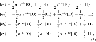
Hence, in the standard computational basis  the eigenvalues can be readily evaluated as

and the corresponding eigenvectors are given by
with 
3. Thermal density and entanglement negativity
The thermal density matrix of the MLGSs at temperature  is given by the Gibbs state

where  and
and  is the partition function. The Boltzmann constant
  is set to
  in this work. The thermal density matrix
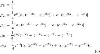
  can be analytically derived by using the spectral decomposition of the Hamiltonian (1). In the two-qubit computational basis, the bipartite density matrix takes the following form:

where the corresponding entries are provided by
The eigenvalues and eigenvectors associated with equation (5) are given by


and
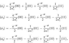
where the asterisk denotes the complex conjugation.
Entanglement negativity leads to the characterization of entanglement for bipartite mixed states in quantum information theory. For the thermal state  of the graphene sheets, which has two sublattices
  and
and  negativity [11, 12] is defined as

where  is the partial transpose of
  with respect to the subsystem
  and
and  is the trace-norm (sum of the singular values) of any arbitrary operator
  The norm
  is typically expressed as

Using equations (5) and (10) in the negativity equation (9), we obtain the analytical expression for negativity which is given by
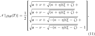
where
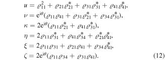
Negativity is presented as a function of temperature in figures 2(a) and (b). It is seen that negativity decreases to zero as the temperature increases. We observe that the threshold temperature can be manipulated by varying the scattering strength and wave number operators. It is interesting that the threshold temperature increases when the scattering parameter  increases. The wave numbers
  and
and  also affect the threshold temperature, but a higher
  results in a slow decrease in negativity and a higher
  shows a rapid decrease in negativity at lower temperature for a given set of parameters.
Figure 2. Negativity ( ) as a function of (a) temperature T for fixed scattering coefficients ω with γ = 1, k
x
= 1 and ky
= 3, (b) temperature T for different values of wave numbers kx
and ky
with ω = 1, γ = 1, (c) the band parameter γ for different wave numbers kx
and ky
with T = 1, ω = 1 and (d) scattering strength ω for various wave numbers kx
and ky
with T = 1, γ = 1. The fixed parameter is μ = π/3.
Download figure:
Standard image High-resolution imageIt is quite obvious that negativity shows a monotonic behavior with the band parameter  and scattering strength
  We observe that negativity is zero when the band parameter
  is zero, and increases with increase in the band parameter
  (figure 2(c)). It is evident that the negativity was generated due to the increase in the band parameter. For higher values of the band parameter
  the negativity reaches the maximum value. On the other hand, the variations of negativity show a very rapid increase for small values of the scattering strength
  from zero to maximum values and decrease with increase of the scattering parameter, as shown in figure 2(d).
4. Quantum correlation quantifiers
LQU and LQFI are both tools used to capture purely quantum correlations in multipartite quantum systems. We introduce LQU and LQFI as quantum correlation quantifiers to examine their behaviors in 2D graphene lattices.
4.1. Local quantum uncertainty
The concept of LQU, the minimum skew information obtained via local measurement on a qubit part, is written as

where  is a Hermitian operator on subsystem
 for the bipartite system and
  is the skew information of the density operator
  which is defined as the so-called Wigner–Yanase skew information [63, 67]

In particular, for bipartite systems, the LQU with respect to subsystem  turns out to be

where 
 and
and  are the eigenvalues of the
  symmetric matrix
  with the entries

and  represents the three Pauli operators of the subsystem
  Using the above method, and after some simplifications, the explicit expressions for the non-vanishing elements of the matrix
  for the 2D graphene lattices are given by


Figure 3 depicts the values of LQU versus temperature  band parameter
  and scattering strength
  respectively. It is quite obvious that LQU shows a monotonic behavior with the band parameter
  and scattering strength
  We observe that LQU is zero when the band parameter
  is zero, and LQU increases with increase in
  It is evident that LQU between the lattice points reaches its maximum value for higher values of
  due to the increase in
  It is very interesting to observe that LQU first increases and then decreases with increase in the wave numbers
  and
and  Furthermore, LQU is maximum at the scattering strength
  and decreases with increase in the scattering strength parameter
  (shown in figure 3(d)) for higher values of both
  and wave numbers
  or
or 
Figure 3. LQU ( ) as a function of (a) temperature T for fixed scattering coefficients ω with γ = 1, kx
= 1 and ky
= 3, (b) temperature T for different values of wave numbers kx
and ky
with ω = 1, γ = 1, (c) band parameter γ for different wave numbers kx
and ky
with T = 1, ω = 1 and (d) scattering strength ω for various wave numbers kx
and ky
with T = 1, γ = 1. The fixed parameter is θ = π/3.
Download figure:
Standard image High-resolution image4.2. Local quantum Fisher information
LQFI, introduced by Girolami et al [63, 64], is recognized as an important key computable measure of a discord-type quantum correlation quantifier in a bipartite quantum system [68].
The measure is defined as the worst-case QFI over all local Hamiltonians  affecting the subspace of party
  in the bipartite system, as follows:

where  We can take the local Hamiltonian as
  with
with 
 is the vector of the Pauli matrices and
  for the bipartite system. After calculation, the analytical form for the LQFI of an arbitrary quantum state for a bipartite system is obtained as

where 
 and
and  are the eigenvalues of the
  real symmetric matrix
  with entries

According to equation (20), we find that the matrix  is diagonal and its eigenvalues are calculated as
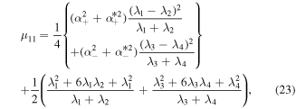


The behavior of LQFI in two-dimensional graphene is plotted in figure 4. Figures 4(a) and (b) show that LQFI is maximal for the temperature  and is reduced by increasing the value of
  In figures 4(c) and (d), we visualize LQFI as a function of the band parameter
  and the scattering strength
  with
with  and
and  Figure 4(c) shows the LQFI versus
  for various values of the wave numbers
  and
and  The LQFI exhibits a sudden change in behavior with
  Indeed, the quantifier of the LQFI displays an increasing behavior until a threshold value
  In addition, increasing
  enhances the number of quantum correlations contained in the system until it reaches a maximum number of correlations. In particular, in figure 4(d) one can see that the LQFI shows an increase in quantum correlations to a maximum value with increasing scattering strength
  until a critical value
  which depends on the values of
  and
and  We notice that the value of the transition point
  increases with increase in the value of
  and
and 
Figure 4. The LQFI ( ) as a function of (a) temperature T for fixed scattering coefficients ω with γ = 1, kx
= 1 and ky
= 3, (b) temperature T for different values of wave numbers kx
and ky
with ω = 1, γ = 1, (c) band parameter γ for various wave numbers kx
and ky
with T = 1, ω = 1 and (d) scattering strength ω for various wave numbers kx
and ky
with T = 1, γ = 1. The fixed parameter is θ = π/3.
Download figure:
Standard image High-resolution image5. Results and discussion
We observe that the negativity, LQU and LQFI show a similar behavior with respect to the three parameters temperature  band parameter
  and scattering coefficient
  as shown in figures 2–4.
Negativity, LQU and LQFI are presented as a function of temperature in figures 2(a), 3(a) and 4(a). It is clearly seen that negativity, LQU and LQFI decrease to zero as the temperature increases. Negativity diminishes more quickly than LQU and LQFI, and it vanishes suddenly. But LQU and LQFI tend to zero asymptotically for large values of temperature. Therefore, LQU and the LQFI appear more stable than negativity. We observe that the threshold temperature can be manipulated by varying the scattering strength and wave number operators. It is interesting that the threshold temperature increases when the scattering parameter increases. Figures 2(b), 3(b) and 4(b) show that the wave numbers  and
and  also affect the threshold temperature, but a higher
  results in a slow decrease in concurrence and a higher
  shows a rapid decrease in concurrence at a lower temperature for a given set of parameters.
The effect of the band parameter  on the behavior of correlation measures is illustrated in figures 2(c), 3(c) and 4(c) for
 Apparently, not all correlations exist for a weak band parameter. They suddenly appear and increase until they obtain steady values and remain in this situation for strong band parameter values. It is clear that
  when they become fixed there are no correlations for weak band parameters
  but with increasing
  they suddenly revive and obtain fixed values for strong
Figures 2(d), 3(d) and 4(d) display the correlations in terms for the scattering strength  for various wave numbers
  and
and  The negativity, LQU and LQFI increase and reach their own maximum values for some weak scattering strength
  The negativity has a lower position than the LQU and LQFI. However, they disappear for strong values of
Skew information (LQU) and LQFI are presented in figures 3 and 4, respectively. Both measures show the same behavior but with different upper bounds. It can be seen that increasing  and
and  has a destructive effect on the non-classical correlations. As depicted in figures 3 and 4, it is obvious that LQU and LQFI exhibit similar variation versus temperature
  Furthermore, it is clear to see from the above results that the amount of quantum correlation measured by LQFI is greater than by LQU. This result agrees with the inequality which states that LQFI is always greater than LQU

6. Conclusion
We employed the negativity, LQU and LQFI criteria for the measurement of quantum correlations in a graphene sheet system. The analytical expressions for negativity, LQU and LQFI were derived. Based on this, the impact of various parameters of the considered system, such as the scattering coefficients and band parameter, wave numbers and temperature on the dynamics of quantum correlations were studied. Our results confirmed that negativity, LQU and LQFI show a similar behavior with respect to the three parameters (temperature, band parameter and scattering coefficients). We observe that at low temperatures negativity remains robust. As the temperature becomes higher, LQFI and LQU remain non-zero, even if negativity vanishes completely. Additionally, we noticed that the degree of non-classical correlations shown by LQFI is always greater than or equal to the LQU. This reveals that the QFI is bounded by the skew information. As a consequence, we think that the presented analysis may offer interesting perspectives for actual and future models in quantum information processing.


