Setting the pace of microswimmers: when increasing viscosity speeds up self-propulsion

It was discovered a few decades ago that many micro-organisms swim faster in more viscous fluids than in less viscous ones. In the first such finding, Shoesmith [1] reported the increased motility of Pseudomonas viscosa, Bacillus brevis and Escherichia coli for a small increase in the viscosity of the solution; larger increases led to the motility decreasing. Similarly, Schneider and Doetsch [2] reported that many flagellated bacteria showed an increase in the velocity when the solution viscosity rose to a characteristic value, and a decrease thereafter. Many other studies [3–6] have corroborated this phenomenon which gainsays both the intuitive expectation of a more viscous fluid providing greater resistance to motion and the traditional theories of microbial motion in simple fluids many of which predict the velocity to go down with the viscosity [7–9].

Theoretical explanations in the past have all focused on the non-Newtonian nature of the fluid and the structure of any polymers present therein, such as the possibility of the latter forming networks inside the fluid which facilitate swimmer propulsion [6, 10–12]. These mechanisms certainly contribute to the anomalous increase of swimmer velocity with fluid viscosity, yet they only concern particular combinations of microswimmer and fluid without attempting to explain the phenomenon in general. Moreover, such explanations suggest that the complex nature of the fluid is essential for the phenomenon to occur.

Here we propose the opposite, by generalizing the explanation to simple, structureless, Newtonian fluids. The central need for complexity in the fluids in the aforementioned explanations lies in the importance of having an interplay between two different time scales in the problem. These time scales stem from the elastic relaxation within the fluid and from the swimming cycle period (defined by the swimming stroke, which is the sequence of shapes that the swimmer adopts in order to propel its motion). Having a fast swimming stroke is not productive if the fluid itself does not relax before the succeeding swimming cycle can commence, and this leads to the existence of an optimal fluid viscosity for a swimmer with an assumed fixed swimming stroke rate. The same reasoning, however, should fit equally well with the motion of a swimmer within a simple Newtonian fluid, as long as there is elasticity in the swimmer body itself. Then the relaxation of the complex fluid can be replaced by the relaxation of any body deformations within the swimmer in the viscous fluid, which again interacts with the stroke time scale to lead to different velocity responses to an increase in the fluid viscosity. For mechanically driven microswimmers, an effective elasticity can be defined assuming the body deformations (including the beating of appendages such as flagella) occur at a steady rate, meaning that they should exhibit both kinds of velocity versus viscosity response.

This argument does not apply to microswimmers whose swimming stroke is predefined, independent of the fluid's influence, as is often the case for theoretical microswimmer models [13–19]. It is well-known that the distance covered by a microswimmer in one swimming cycle is proportional to the area of the closed loop in configuration space that its swimming stroke describes [20, 21]. The effect of the different forces acting on the swimmer is subsumed in the swimming stroke, meaning that when the latter is imposed then the effect of force parameters such as the viscosity is lost. (As illustration, see the velocity expressions for four prominent microswimmer models in [15, 17, 22, 23], each of which depends solely on the respective swimmer's geometrical parameters and the prescribed swimming stroke.) Hence, to see the full dependence of the swimming velocity on the fluid viscosity, a force/energy-centric approach, which allows the swimmer to adjust its swimming stroke in response to the driving, is necessary.

To test the above general argument, we perform an analytical and numerical study of a mechanical microswimmer in a simple Newtonian fluid, based on the popular three-sphere model of Najafi and Golestanian [13]. In the three-sphere model the swimming stroke is imposed and the swimmer consequently does not exhibit a velocity dependence on the fluid viscosity [13, 23]. Our purposes therefore require us to modify this model, by including springs between the spheres and imposing the forces driving the motion instead of the swimming stroke, allowing the latter to emerge in response to the former. This reworked model is amenable to fully analytical treatment. Moreover, since the swimmer is driven by only two elastic degrees of freedom, the simplicity of the design allows one to generalize the results to other microswimmers which are driven by elastic components.

Analysis of the model confirms the fact that two regimes of motion exist, in one of which the swimmer gets slower (which we call the 'conventional' regime) and in the other one faster (the 'aberrant' regime) when the viscosity of the surrounding fluid is increased. The regimes depend on a ratio Γ  of two characteristic time scales,

$$\begin{eqnarray}&&{\rm{\Gamma }}=\displaystyle \frac{\mathrm{relaxation}\ \mathrm{time}\ \mathrm{of}\ \mathrm{spheres}\ \mathrm{in}\ \mathrm{fluid}}{\mathrm{swimming}\ \mathrm{cycle}\ \mathrm{period}}.\end{eqnarray} \tag{ 1.1 }$$

Assume that the swimming cycle period is fixed. For ${\rm{\Gamma }}\gg 1$ the spheres do not relax fully within one swimming cycle, and increasing the fluid viscosity causes them to relax even less, making the swimmer swim slower. For ${\rm{\Gamma }}\ll 1$ the spheres relax very quickly, but that is not advantageous since the swimming speed is limited by the cycle period. Moreover, a quick relaxation rate of the spheres (concomitant with a small fluid viscosity) also reduces the inter-sphere hydrodynamic interactions which are vital to the swimming motion. Therefore in this case increasing the fluid viscosity leads to faster swimming. This whole picture can be seen from the reverse point of view, where Γ  is modified by changing the swimming cycle period instead of the sphere relaxation time. As shown in a previous work [24], the swimming velocity shows a maximum as a function of the cycle frequency, because for very quick driving the spheres do not relax within one cycle, and in the limit of very slow driving the swimming tends to cease. Note that this rate-dependence of the swimming velocity disappears in the Stokesian realm once the stroke is imposed (apart from an overall scaling factor of the frequency), since there is then only one characteristic time scale in the problem.

The dependence of the aberrant swimming phenomenon on the sphere (or, more generally, body deformation) relaxation time speaks immediately to the necessity of having an elastic degree of freedom in the swimmer which couples to the fluid viscosity to determine the rate of relaxation. Lastly, since the aberrant regime is observed for small viscosities, then for the low Reynolds number condition of microswimming to be honored, the driving (and hence the motion velocity) needs to be weak.

The swimmer consists of three beads connected in series by two harmonic springs (figure 1), and driven by known forces of the form

$$\begin{eqnarray}{{\bf{F}}}_{1}^{{\rm{d}}}(t) & = & A\sin (\omega t)\hat{{\bf{z}}},\\ {{\bf{F}}}_{2}^{{\rm{d}}}(t) & = & -{{\bf{F}}}_{1}^{{\rm{d}}}(t)-{{\bf{F}}}_{3}^{{\rm{d}}}(t),\ \mathrm{and}\\ {{\bf{F}}}_{3}^{{\rm{d}}}(t) & = & B\sin (\omega t+\alpha )\hat{{\bf{z}}},\ \mathrm{with}\ \alpha \in [-\pi ,\pi ].\end{eqnarray} \tag{ 2.1 }$$

Here A and B are non-negative amplitudes of the time-dependent driving forces ${{\bf{F}}}_{1}^{{\rm{d}}}(t)$ and ${{\bf{F}}}_{3}^{{\rm{d}}}(t)$ applied along the $\hat{{\bf{z}}}$-direction to the outer beads at the frequency ω and with the phase difference α. The force ${{\bf{F}}}_{2}^{{\rm{d}}}(t)$ on the middle bead is set by the condition for autonomous propulsion, which requires the net driving force on the device to vanish at all times. The two springs are identical, with a stiffness constant k and a rest length l which is much larger than the bead dimensions. For convenience, we define a 'reduced friction coefficient' λ of the beads as

$$\begin{eqnarray}&&\lambda =\displaystyle \frac{\gamma }{6\pi \eta },\end{eqnarray} \tag{ 2.2 }$$

where γ is their Stokes drag coefficient and η is the dynamic viscosity of the fluid. The parameter λ has dimensions of length and plays the role of the radius for non-spherical beads [24].

Zoom In Zoom Out Reset image size

For our swimmer the ratio of time scales Γ  becomes

$$\begin{eqnarray}&&{\rm{\Gamma }}={\tau }_{{\rm{s}}}\ \omega =\displaystyle \frac{6\pi \omega \lambda \eta }{k},\end{eqnarray} \tag{ 2.3 }$$

where ${\tau }_{{\rm{s}}}$ is the relaxation time of the spheres in the fluid, defined as

$$\begin{eqnarray}&&{\tau }_{{\rm{s}}}=\displaystyle \frac{\gamma }{k}=\displaystyle \frac{6\pi \lambda \eta }{k}.\end{eqnarray} \tag{ 2.4 }$$

The fluid is assumed to be governed by the Stokes equation

$$\begin{eqnarray}&&\eta {{\rm{\nabla }}}^{2}{\bf{u}}({\bf{r}},t)-{\rm{\nabla }}p({\bf{r}},t)+{\bf{f}}({\bf{r}},t)={\bf{0}},\end{eqnarray} \tag{ 2.5 }$$

and the incompressibility condition

$$\begin{eqnarray}&&{\rm{\nabla }}\cdot {\bf{u}}=0.\end{eqnarray} \tag{ 2.6 }$$

Here ${\bf{u}}({\bf{r}},t)$ and $p({\bf{r}},t)$ are the velocity and the pressure of the fluid at the point ${\bf{r}}$ at time t. The force density ${\bf{f}}({\bf{r}},t)$ acting on the fluid, in the limit of small bead dimensions, is given by

$$\begin{eqnarray}&&{\bf{f}}({\bf{r}},t)=\displaystyle \sum _{i=1}^{3}[{{\bf{F}}}_{i}^{{\rm{d}}}(t)+{{\bf{F}}}_{i}^{{\rm{s}}}(t)]\delta ({\bf{r}}-{{\bf{R}}}_{i}(t)),\end{eqnarray} \tag{ 2.7 }$$

where the index $i=1,2,3$ denotes the ith bead placed at the position ${{\bf{R}}}_{i}(t)$ subject to a driving force ${{\bf{F}}}_{i}^{{\rm{d}}}(t)$ and a spring force ${{\bf{F}}}_{i}^{{\rm{s}}}(t)$ (which, for the middle bead, results from two springs). Here $\delta ({\bf{r}})$ denotes the Dirac delta function. Assuming no slip at the fluid-bead interfaces, the instantaneous velocity ${{\bf{v}}}_{i}(t)$ of each bead [25] is given by

$$\begin{eqnarray}&&{{\bf{v}}}_{i}=\displaystyle \frac{{\rm{d}}{{\bf{R}}}_{i}}{{\rm{d}}t}=({{\bf{F}}}_{i}^{{\rm{d}}}+{{\bf{F}}}_{i}^{{\rm{s}}}){\gamma }^{-1}+\displaystyle \sum _{j\ne i}{\bf{T}}({{\bf{R}}}_{i}-{{\bf{R}}}_{j})\cdot ({{\bf{F}}}_{i}^{{\rm{d}}}+{{\bf{F}}}_{i}^{{\rm{s}}}),\end{eqnarray} \tag{ 2.8 }$$

where ${\bf{T}}({\bf{r}})$ is the Oseen tensor [26, 27], and is here diagonal due to the collinear nature of the driving forces and the employed far-field approximation (which assumes that the bead dimensions are much smaller than l).

In the steady state the bead positions are of the form [28]

$$\begin{eqnarray}&&{{\bf{R}}}_{i}(t)={{\bf{S}}}_{i0}+{{\boldsymbol{\xi }}}_{i}(t)+{\bf{v}}t\end{eqnarray} \tag{ 2.9 }$$

due to the sinusoidal nature of the forces. Here ${{\boldsymbol{\xi }}}_{i}(t)$ denotes small sinusoidal oscillations around the uniformly moving equilibrium configuration ${{\bf{S}}}_{i0}+{\bf{v}}t$, where ${{\bf{S}}}_{i0}$ are the initial positions of the beads and ${\bf{v}}$ is the mean cycle-averaged uniform swimming velocity of the assembly. Clearly we have $| {{\bf{S}}}_{20}-{{\bf{S}}}_{10}| =| {{\bf{S}}}_{30}-{{\bf{S}}}_{20}| =l$.

Equations (2.8) and (2.9) lead to a coupled system of differential equations in the ${{\boldsymbol{\xi }}}_{i}$'s, which can be solved by a perturbative scheme by expanding the functions of the arm-lengths $| {{\bf{R}}}_{2}(t)-{{\bf{R}}}_{1}(t)|$ and $| {{\bf{R}}}_{3}(t)-{{\bf{R}}}_{2}(t)|$ around their mean values l, if we assume that the driving forces, and consequently the oscillations ${{\boldsymbol{\xi }}}_{i}(t)$, are small, i.e. $| {{\boldsymbol{\xi }}}_{i}(t)| \ll l$ for all i and all times t [28, 29]. The functions expanded are ${\bf{T}}({{\bf{R}}}_{i}(t)-{{\bf{R}}}_{j}(t))$ and ${\bf{G}}({{\bf{R}}}_{i}(t)-{{\bf{R}}}_{j}(t))$ (appendix A.1), where the latter are the pairwise spring forces between two neighboring beads [29],

$$\begin{eqnarray}&&{\bf{G}}({{\bf{R}}}_{i}(t)-{{\bf{R}}}_{j}(t))=-k\left(\displaystyle \frac{{{\bf{R}}}_{i}({\bf{t}})-{{\bf{R}}}_{j}({\bf{t}})}{| {{\bf{R}}}_{i}(t)-{{\bf{R}}}_{j}(t)| }\right)(| {{\bf{R}}}_{i}(t)-{{\bf{R}}}_{j}(t)| -l),\end{eqnarray} \tag{ 2.10 }$$

such that the total spring force on the $i\mathrm{th}$ bead can be expressed as

$$\begin{eqnarray}&&{{\bf{F}}}_{i}^{{\rm{s}}}(t)=\displaystyle \sum _{j\ne i}^{3}{\bf{G}}({{\bf{R}}}_{i}(t)-{{\bf{R}}}_{j}(t)).\end{eqnarray} \tag{ 2.11 }$$

Since the forces and the displacements are all sinusoidal, the first-order terms in the velocity ${\bf{v}}$ (in terms of the perturbation variable ${{\boldsymbol{\xi }}}_{i}(t)$) integrate to 0 over a swimming cycle. We calculate to the second order in ${{\boldsymbol{\xi }}}_{i}/l$, therefore, and find the velocity expression for the swimmer to be

$$\begin{eqnarray}&&{\bf{v}}=\displaystyle \frac{7\omega \lambda [{AB}({k}^{2}+12{\pi }^{2}{\omega }^{2}{\eta }^{2}{\lambda }^{2})\sin \alpha +2\pi ({A}^{2}-{B}^{2})k\omega \eta \lambda ]}{24{l}^{2}({k}^{2}+4{\pi }^{2}{\omega }^{2}{\eta }^{2}{\lambda }^{2})({k}^{2}+36{\pi }^{2}{\omega }^{2}{\eta }^{2}{\lambda }^{2})}\hat{{\bf{z}}}.\end{eqnarray} \tag{ 2.12 }$$

This expression, being a non-monotonic function of the viscosity η, directly shows the existence of the conventional and aberrant velocity–viscosity regimes. Note that both these regimes are obtained if we let one of the driving force amplitudes A and B be zero, i.e. when the swimmer has one active and one passive elastic degree of freedom.

We now study these regimes by changing only the viscosity η and keeping all the other independent parameters in the problem fixed, including the driving forces. An alternative approach would be to vary the driving forces such that the efficiency of the compared swimmers is held constant. Fixing the driving forces is easier, and the results for constant efficiencies would be essentially the same since the efficiencies of fast swimmers are generally higher than those of slow ones [24, 30].

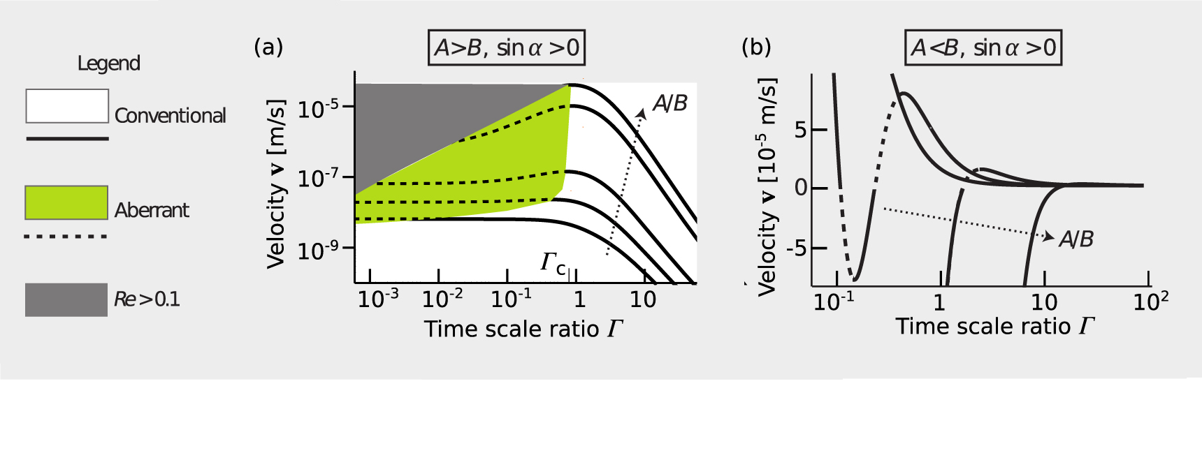
We find that when $(A-B)/\sin \alpha \gt 0$, then the velocity ${\bf{v}}$ as a function of η has exactly one extremum (see figure 2(a), where Γ  plays the role of a dimensionless viscosity since all the factors except η in equation (2.3) are held constant). This extremum divides the conventional regime, obtained for large viscosities and shown in white in figure 2(a), and the aberrant regime, obtained for small viscosities and shown in green (light gray in grayscale print). The different curves correspond to increasing values of A, with B constant. Some manipulation of the velocity expression shows that for each curve the swimmer lies in the conventional regime if

$$\begin{eqnarray}&&{\rm{\Gamma }}\gt {{\rm{\Gamma }}}_{{\rm{c}}}=\displaystyle \frac{3}{\sqrt{5+2\sqrt{13}}}\approx 0.86.\end{eqnarray} \tag{ 3.1 }$$

Zoom In Zoom Out Reset image size

The dark gray area marks the region where the swimmer Reynolds number Re > 0.1 (where ${Re}\,=\,| {\bf{v}}| l\rho /\eta$, with ρ denoting the fluid density), when we assume the condition of Stokes flow to be violated. For large enough values of the driving force amplitude A, the entire part of the velocity curve for which ${Re}\,\lt \,0.1$ falls in the conventional regime.

If $(A-B)/\sin \alpha \lt 0$, then the velocity can have several local extrema (figure 2(b)). Moreover, the swimmer can reverse direction if the fluid viscosity is changed. If the force parameters satisfy the condition

$$\begin{eqnarray}&&\displaystyle \frac{B}{A}\gt \sqrt{1+6{\sin }^{2}\alpha +2\sin \alpha \sqrt{3+9{\sin }^{2}\alpha }},\end{eqnarray} \tag{ 3.2 }$$

then the swimmer becomes aberrant for an intermediate range of viscosities (dashed parts of curves in figure 2(b)).

To depict the importance of the time scale ratio Γ in controlling the regime of motion, we fix in figure 3 the fluid viscosity η and change Γ by varying the spring stiffness k. The different plots in figure 3 mark the conventional and the aberrant regimes for different values of the driving force parameters A, B and α, and for decreasing Γ. At large Γ  values, the conventional regime is dominant (leftmost panel in figure 3). In the limit of infinite Γ, which corresponds to zero elasticity (k = 0), the whole phase space is conventional, as is easily seen by putting k = 0 in equation (2.12). This is because then the spheres never relax back from any displacement and there is no competition of time scales in the problem. As Γ  decreases, the relative area of the aberrant regime rises continuously (center left panel in figure 3) as long as the inequality (3.1) is satisfied. At the critical value ${\rm{\Gamma }}={{\rm{\Gamma }}}_{{\rm{c}}}(\approx 0.86)$, there is a discontinuous change in the nature of the regimes across most of the phase space, with the aberrant regime becoming dominant (center right and right panels in figure 3). This recalls our earlier discussion of the swimming being aberrant for small values of Γ.

Zoom In Zoom Out Reset image size

To confirm the existence of the two viscosity-dependent regimes that the theory predicts, we employ numerical simulations (commonly used to study micro-swimming; see [31–49]). For this we use the LB3D code [35, 50] based on the immersed-boundary method (IBM) and the lattice-Boltzmann method (LBM) [51]. We run two sets of simulations (details provided in appendix A.2), to account for both the cases of $(A-B)/\sin \alpha \gtrless 0$ (figure 4). In both the investigated sets we observe that the two predicted velocity–viscosity regimes are reproduced well. The small errors are attributable to the unrealizably small radius to arm-length ratios in the theoretical model, in addition to the limitations inherent in simulations (such as boundary effects and imperfect space and time discretization).

Zoom In Zoom Out Reset image size

In this work we have shown that for a fluid-active particle system involving an elastic degree of freedom, the competition between the characteristic time scales associated with the driving and with the elastic relaxation is sufficient for a non-monotonic velocity–viscosity response. In the present study, we assume that it is the swimmer that possesses a responsive elastic degree of freedom, as is the case for most microswimmer models and real swimmers such as those driven by flagella. In contrast, the requisite elasticity may be provided by the fluid, in which case equivalent response is found [6, 10–12] since the physical principle involved is similar.

We have tested our argument by calculating analytically the velocity of a bead-spring microswimmer driven by sinusoidal forces. We have shown that the swimmer exhibits both the conventional and the aberrant kinds of behavior (defined as a decrease and an increase, respectively, of the swimming velocity with the fluid viscosity) for expected ranges of the time scale ratio. The minimality of the model, consisting of only two elastic degrees of freedom and a Newtonian continuum as the fluid, promotes the idea that similar behavior should be exhibited by other swimmer models. The theoretical results are confirmed by independent and closely agreeing lattice-Boltzmann simulations.

Previous studies in the literature have looked at the contrasting effects of elastic forces and viscous forces when the swimmer's elasticity is changed. For instance, the swimming speed as a function of the Sperm number Sp (or equivalently, the elastohydrodynamic penetration length) of an elastic filament has been shown to exhibit a maximum [52, 53], with Sp varied by changing the bending modulus of the filament. More recently, it has been found that the Schistosoma mansoni parasite maintains a flexibility at its tail-fork joint near a value which optimizes its swimming efficiency [54]. This flexibility is modeled in the theory as the stiffness of a torsional spring at the tail-fork joint, and results in a similar time scale ratio as our Γ having a value of 1 for the optimum swimming velocity. These studies are evidence of the generality of our description of how the viscous and the elastic time scales interact and affect swimming.

The interplay of different time scales may result in qualitative effects on the swimming motion, in addition to affecting the swimming speed. For instance, for beating flagella, the radius of curvature has been found to change when the fluid viscosity is increased [55], and the power and recovery strokes have been shown to accelerate and decelerate, respectively, upon loading by external flows [56]. If the system contains additional time scales then there is also a possibility of more complicated velocity–viscosity regimes. In this context, it would be interesting to see if, and how, active fluctuations in the fluid [57] and stochastic stroke modulation by the swimmer [58, 59] can modulate the relationship between the swimming velocity and the fluid viscosity.

In conclusion, our work here has highlighted a general feature of mechanical microswimming, drawing on the way that the viscosity of any fluid interacts with the elasticity of the system. On a fundamental level, it is a further testament to the fact that motion at the micro- (and smaller) scales is non-trivial and that 'resistance' at these scales can often be beneficial for motion [24, 60, 61].

A-SS and JP thank the funding of the European Research Council through the grant MembranesAct ERC Stg 2013-337283, and of the Deutsche Forschungsgemeinschaft (DFG) through the Cluster of Excellence: Engineering of Advanced Materials. J H acknowledges support by NWO/STW (Vidi grant 10787) and LM thanks the DAAD for a RISE scholarship. TK thanks the University of Edinburgh for the award of a Chancellor's Fellowship.

A.1. Expansions of the Oseen tensor and the spring forces to the $1\mathrm{st}$ order in the oscillations around the equilibrium configuration

The expansions of ${\bf{T}}({{\bf{R}}}_{i}(t)-{{\bf{R}}}_{j}(t))$ and ${\bf{G}}({{\bf{R}}}_{i}(t)-{{\bf{R}}}_{j}(t))$ (in equations (2.8) and (2.10)) to the first order in $({{\boldsymbol{\xi }}}_{i}(t)-{{\boldsymbol{\xi }}}_{j}(t))$ may be found in [29], and are provided here for the sake of completeness.

$$\begin{eqnarray}&&{\bf{T}}({{\bf{R}}}_{i}(t)-{{\bf{R}}}_{j}(t))=\quad {\bf{T}}({{\bf{R}}}_{i}(0)-{{\bf{R}}}_{j}(0))+{\displaystyle \frac{\partial {\bf{T}}({{\bf{R}}}_{i}(t)-{{\bf{R}}}_{j}(t))}{\partial {{\bf{R}}}_{i}(t)}\bigg|}_{t=0}\cdot ({{\boldsymbol{\xi }}}_{i}(t)-{{\boldsymbol{\xi }}}_{j}(t))\\ &&\quad ={{\bf{T}}}_{{ij}}+{{\bf{P}}}_{{ij}}\cdot ({{\boldsymbol{\xi }}}_{i}(t)-{{\boldsymbol{\xi }}}_{j}(t)),\ \mathrm{with}\ {{\bf{T}}}_{{ij}}={\bf{T}}({{\bf{R}}}_{i}(0)-{{\bf{R}}}_{j}(0))\ \mathrm{and}\ {{\bf{P}}}_{{ij}}={\displaystyle \frac{\partial {\bf{T}}({{\bf{R}}}_{i}(t)-{{\bf{R}}}_{j}(t))}{\partial {{\bf{R}}}_{i}(t)}\bigg|}_{t=0},\end{eqnarray} \tag{ A.1.1 }$$

and

$$\begin{eqnarray}&&{\bf{G}}({{\bf{R}}}_{i}(t)-{{\bf{R}}}_{j}(t))\,=\\ &&\quad {\bf{G}}({{\bf{R}}}_{i}(0)-{{\bf{R}}}_{j}(0))+{\displaystyle \frac{\partial {\bf{G}}({{\bf{R}}}_{i}(t)-{{\bf{R}}}_{j}(t))}{\partial {{\bf{R}}}_{i}(t)}\bigg|}_{t=0}\cdot ({{\boldsymbol{\xi }}}_{i}(t)-{{\boldsymbol{\xi }}}_{j}(t))\\ &&\quad ={{\bf{H}}}_{{ij}}\cdot ({{\boldsymbol{\xi }}}_{i}(t)-{{\boldsymbol{\xi }}}_{j}(t)),\ \mathrm{with}\ {{\bf{H}}}_{{ij}}={\displaystyle \frac{\partial {\bf{G}}({{\bf{R}}}_{i}(t)-{{\bf{R}}}_{j}(t))}{\partial {{\bf{R}}}_{i}(t)}\bigg|}_{t=0}.\end{eqnarray} \tag{ A.1.2 }$$

A.2. Details of the different simulations presented in figure 4

A.3. Velocity expression for unequal spring constants

To highlight a case when a symmetric driving of the swimmer results in a non-reciprocal swimming stroke and consequently swimming, we here present the velocity expression for our swimmer model if the two springs are allowed to have different stiffness constants k₁ and k₂. The calculation is similar to that leading to equation (2.12), and gives the result

$$\begin{eqnarray}&&{\bf{v}}=\displaystyle \frac{7\omega \lambda \{{AB}[({k}_{1}{k}_{2}+12{\pi }^{2}{\omega }^{2}{\eta }^{2}{\lambda }^{2})\sin \alpha +4({k}_{2}-{k}_{1})\pi \omega \eta \lambda \cos \alpha ]+2\pi ({A}^{2}{k}_{2}-{B}^{2}{k}_{1})\omega \eta \lambda ]}{24{l}^{2}[{k}_{1}^{2}{k}_{2}^{2}+8(2{k}_{1}^{2}+2{k}_{2}^{2}+{k}_{1}{k}_{2}){\pi }^{2}{\omega }^{2}{\eta }^{2}{\lambda }^{2}+144{\pi }^{4}{\omega }^{4}{\eta }^{4}{\lambda }^{4}]}\hat{{\bf{z}}}.\end{eqnarray} \tag{ A.3.1 }$$

It may easily be checked that the above velocity expression reduces to equation (2.12) for ${k}_{1}={k}_{2}=k$, gives a zero velocity if either of the k_i's is infinite (for then the swimmer is akin to a two bead swimmer), and results in a non-zero swimming velocity for symmetric driving, i.e. if A = B and $\alpha =0$, unlike the expression in equation (2.12). A similar swimmer, with symmetric driving but unequal spring stiffnesses, has been recently realized experimentally [63].

If the individual relaxation rates of the two springs are considered, then an additional time scale ratio in the problem must be introduced. This makes the dependence of the velocity on the viscosity more elaborate but does not affect the existence of the conventional and the aberrant swimming regimes.