


Abstract
We present a feasible proposal for quantum tomography of qubit and qutrit states via mutually unbiased measurements in dispersively coupled driven cavity QED systems. We first show that measurements in the mutually unbiased bases (MUBs) are practically implemented by projecting the detected states onto the computational basis after performing appropriate unitary transformations. The measurement outcomes can then be determined by detecting the steady-state transmission spectra (SSTS) of the driven cavity. It is found that all the measurement outcomes for each MUB (i.e., all the diagonal elements of the density matrix of each detected state) can be read out directly from only one kind of SSTS. In this way, we numerically demonstrate that the exemplified qubit and qutrit states can be reconstructed with the fidelities 0.952 and 0.961, respectively. Our proposal could be straightforwardly extended to other high-dimensional quantum systems provided that their MUBs exist.
Export citation and abstract BibTeX RIS

Original content from this work may be used under the terms of the Creative Commons Attribution 3.0 licence. Any further distribution of this work must maintain attribution to the author(s) and the title of the work, journal citation and DOI.
1. Introduction
One of the essential tasks in quantum information processing is how to extract the complete information of an unknown quantum state. A powerful method to achieve this aim is known as quantum state tomography (QST), i.e., reconstructing the density matrix of this unknown quantum state [1]. Due to its particular importance in quantum information processing, QST has received considerable attention in recent decades, and a great deal of significant advancements have been achieved in theoretical [2–7] and experimental aspects [8–12].
In order to realize QST, one first needs to perform a series of projective measurements on a large enough number of identically prepared copies of the quantum state, and then reconstructs its density matrix from these measurement outcomes. Prior to measurements, a crucial issue is the choice of measurement sets [13]. To increase the accuracy and efficiency in QST, several kinds of measurement sets have been explored and employed, including the set of the measurement bases, e.g., standard projective measurement bases [2, 3], equidistant states [14], symmetric informationally complete positive operator-valued measures [15, 16], mutually unbiased bases (MUBs) [17], and so on.
MUBs are a typical kind of measurement bases, which are defined by the property that the squared overlaps between a basis state in one basis and all basis states in the other bases are the same [17]. Physically, this means that the measurement of a particular basis state does not reveal any information about the state if it was prepared in another basis. Due to this distinct property, MUBs have extensive applications in the field of quantum information. Therein, a typical application is QST [18–23]. In the context of QST, Wootters and Fields [18] proved that the measurements in the MUBs provide a minimal and optimal way to realize QST (called MUBs-QST hereafter) in the sense of maximizing information extraction from each measurement and minimizing the effects of statistical errors in the measurements. By far, several experiments have been demonstrated to implement MUBs-QST only in optical systems [24–27]. Additionally, a theoretical scheme has been presented to realize MUBs-QST of two spin qubits in a double quantum dot [28].
As a possible physical implementation, in this paper we propose a feasible proposal for MUBs-QST in dispersively coupled driven cavity QED systems. We demonstrate our idea for the cases of qubit and qutrit states. Certainly, our idea is also suitable for other high-dimensional quantum systems if their MUBs exist. The main idea of our proposal is summarized as follows. First, measurements in the MUBs are implemented by projecting the detected states onto the computational basis after performing proper unitary transformations, which can be readily realized by adjusting the classical driving field applied on the qubit or qutrit. Secondly, the projective measurement outcomes can be determined by detecting the steady-state transmission spectra (SSTS) of the driven cavity. Through theoretical analysis and numerical experiments, it is found that multiple peaks appear in the SSTS: each of the detected peaks marks one of the computational basis states and its relative height equals the corresponding superposed probability in the detected state. This manifest advantage allows us to directly read out all the measurement outcomes for each MUB (i.e., all the diagonal elements of the density matrix of each detected state) by only one kind of SSTS. In this manner, MUBs-QST can be realized. Finally, our proposed readout method is of the nondestructive property [29]. This means that what we directly detect is the transmitted photons through the driven cavity, rather than intracavity atom itself. The measurement-induced noises on the atom can be efficiently suppressed. Thus we numerically demonstrate that the fidelities of the exemplified qubit and qutrit states can attain 0.952 and 0.961, respectively.
The rest of this paper is organized as follows. In section 2, we briefly introduce the MUBs and the MUBs-QST for d-dimensional quantum system, especially for two minimal prime numbers d = 2 and d = 3. In section 3, we show in detail how to realize the required unitary transformations, the SSTS, and further MUBs-QST of qubit states with them. The extension to the case of qutrit states is explicitly shown in section 4. Discussion on the experimental implementation of our proposal is given in section 5. This paper ends up with a conclusion in section 6.
2. MUBs and MUBs-QST
In a d-dimensional quantum system, two orthogonal bases  and
and  are defined as MUBs if and only if any pair of basis states from different orthogonal bases (
 ) satisfy [17]

where  labels one of the basis states in the
  th orthogonal basis. It is known that the number of MUBs for any dimension d is at most
  [18], and exactly
  if the dimension d is a prime [19] or a power of a prime [18]. Such
  MUBs constitute a complete set if each pair of MUBs in this set is mutually unbiased [18]. Nevertheless, whether a complete set of MUBs exists or not in other finite dimensions is still unknown, for instance, d = 6 [30–32].
It is well known that the measurements in the MUBs provide a minimal and optimal way to completely determine the density matrix of an unknown quantum state [18]. In terms of the MUBs, the density matrix of an arbitrary d-dimensional quantum state can be represented as [19]

where the MUBs-projector  defines a complete set of projective measurements,
  is the probability of projecting
  onto the basis state
  of the kth MUB, and I is an identity operator. The measured probability can be equivalently written as

where Udk is the unitary transformation that transforms the standard computational basis  into the kth MUB in a d-dimensional quantum system. From equation (3), it can be seen that the measurements in the MUBs can be realistically implemented by projecting the detected state onto the computational basis after performing appropriate unitary transformations
  . And the projective measurement outcome
  is exactly the value of the diagonal element
  of the transformed density matrix
  . With these projective measurement outcomes, the MUBs-QST can be realized.
Specifically, we show the correspondence between the measurements in the kth MUB and the required unitary transformations Vdk for d = 2 and d = 3 in table 1. Therein,  is the Hadamard gate,
  with the Pauli operator
  , F is the Fourier transformation with the effect of
  and
and  is its inverse operator,
 is the phase operation and
  is its inverse operator.
Table 1. The correspondence between the measurement in the kth MUB and the required unitary transformation Vdk for d = 2 and d = 3, respectively. See the text for details.
| d = 2 | d = 3 | ||
|---|---|---|---|
| k | V2k | k | V3k |
| 1 | I | 1 | I |
| 2 |

|
2 |

|
| 3 |

|
3 |

|
| 4 |

|
||
3. MUBs-QST of qubit states
3.1. Implementation of single-qubit unitary transformations
We consider a cavity QED system sketched in figure 1(a), wherein a qubit (two-level atom) shown in figure 1(b) is dispersively coupled to a cavity. In order to implement single-qubit unitary transformations, we only need to add a classical driving field on the qubit, see figure 1(b). Under the rotating-wave approximation, the whole system can be described by the Hamiltonian ( hereafter the same)

where  is the cavity frequency,
  is the creation (annihilation) operator of the cavity photon,
  is the transition frequency of the qubit with the Pauli operators:
  ,
,  , and
, and  , g is the coupling strength between the qubit and the cavity, Ω and ν are the amplitude and the frequency of the classical driving field.
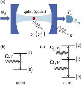
Figure 1. (a) Schematic diagram of a cavity QED system, wherein a qubit (two-level atom) or a qutrit (three-level atom) is dispersively coupled to a cavity. The qubit or qutrit states can be nondestructively read out by applying a classical driving field with the frequency  on one side of the cavity and then detecting its SSTS Tss on the other side. κ denotes the photon decay rate of the cavity,
  the qubit decay rate,
 the qutrit decay rates. (b) A classical driving field with the amplitude Ω and the frequency ν is applied on the qubit to implement the required single-qubit unitary transformations. (c) Two classical driving fields with the amplitude
  and the frequency
  , and the amplitude
  and the frequency
  , are applied between the energy levels
  and
and  , and between
  and
and  , respectively, to realize the required single-qutrit unitary transformations.
Download figure:
Standard image High-resolution imageIn a frame rotating at the frequency ν of the classical driving field for both the qubit and the cavity, the Hamiltonian (4) is changed to

with  being the frequency detuning of the cavity from the classical driving field, and
  being the frequency detuning of the qubit from the classical driving field.
Similar to [33], in the dispersive regime (i.e.,  with
with  ), we perform the unitary transformation
 ![$U=\mathrm{exp}[g({a}^{\dagger }{\sigma }_{-}-a{\sigma }_{+})/{\rm{\Delta }}]$](https://content.cld.iop.org/journals/1367-2630/18/4/043013/revision1/njpaa1d45ieqn54.gif) on the Hamiltonian (5) to eliminate the direct qubit-cavity coupling. Using the Hausdorff expansion to second order in the small parameter
on the Hamiltonian (5) to eliminate the direct qubit-cavity coupling. Using the Hausdorff expansion to second order in the small parameter  , the effective Hamiltonian reads as

where  with
with  . As the average photon number of the cavity
  , this Hamiltonian (6) can generate rotations of the qubit about any axis on the Bloch sphere by adjusting the frequency ν of the classical driving field. First, if we adjust
  so that
  , the rotations of the qubit around x axis on the Bloch sphere can be generated, that is, the unitary transformation
  with
with  . Therefore, the required unitary transformation
  can be implemented with the duration time
  . Secondly, if the driving frequency is adjusted as
  , we can realize the required Hadamard gate
  with the duration time
  . Finally, the combination of
  and
and  can generate rotations of the qubit about z axis on the Bloch sphere since
  , and the total duration time is
  .
.
3.2. SSTS of a driven cavity with a qubit
For the readout of the qubit states, we need to apply another classical driving field on one side of the cavity, and then detect its SSTS on the other side, see figure 1(a). The interaction Hamiltonian between the applied driving and the cavity reads as

where  is the time-independent real amplitude and
  is the frequency of the applied driving. The total Hamiltonian HT of such a driven cavity-qubit system includes Hd plus the first three terms of equation (4). In the dispersive regime and in a frame rotating at the driving frequency
  for the cavity, the effective Hamiltonian of the whole system is derived as

where  is the detuning between the driving frequency and the cavity frequency.
Under the Born–Markov approximation, the dynamics of the whole system is governed by the master equation [29]

where ρ is the density matrix of the system and ![${ \mathcal D }[{\mathbb{A}}]\rho ={\mathbb{A}}\rho {{\mathbb{A}}}^{\dagger }-{{\mathbb{A}}}^{\dagger }{\mathbb{A}}\rho /2-\rho {{\mathbb{A}}}^{\dagger }{\mathbb{A}}/2$](https://content.cld.iop.org/journals/1367-2630/18/4/043013/revision1/njpaa1d45ieqn75.gif) . Here,
. Here,  is the qubit energy decay rate,
  the qubit dephasing rate, and κ the photon decay rate of the cavity. From the master equation (9), the coupled equations of motion related to the desired quantity
  are given by


with  . From equation (10d), we can obtain
 ![$\langle {\sigma }_{z}({t}_{{\rm{NDR}}})\rangle ={{\rm{e}}}^{-{\gamma }_{1}{t}_{{\rm{NDR}}}}[\langle {\sigma }_{z}(0)\rangle +1]-1\simeq \langle {\sigma }_{z}(0)\rangle $](https://content.cld.iop.org/journals/1367-2630/18/4/043013/revision1/njpaa1d45ieqn80.gif) since
since  and
and  [34], where the subscript NDR denotes nondestructive readout. Further, the normalized SSTS
  of the driven cavity is analytically derived from equations (10a)–(10c) as

where the subscript ss denotes steady state.
From equation (8), it can be seen that the interaction Hamiltonian between the qubit and the cavity is  , which commutes with the qubit operator
  , i.e.,
 ![$[{H}_{\mathrm{int}},{\sigma }_{z}]=0$](https://content.cld.iop.org/journals/1367-2630/18/4/043013/revision1/njpaa1d45ieqn86.gif) . Therefore, the transmission spectra readout method proposed above is of the nondestructive property [29]. The interaction Hamiltonian Hint also indicates that the cavity frequency is shifted by
. Therefore, the transmission spectra readout method proposed above is of the nondestructive property [29]. The interaction Hamiltonian Hint also indicates that the cavity frequency is shifted by  (or L), if the qubit is in the computational basis state
  (or
(or  ). Hence, the shifts of the cavity frequency can mark the computational basis states of the qubit. On the other hand, only the incident photon whose frequency is equivalent to one of the state-dependent frequencies
  of the cavity can transmit the cavity and then be detected. Physically, the detected probability is exactly the superposed probability of the computational basis state in the qubit state. Therefore, the SSTS Tss (11) has the feature: the relative height of each transmitted peak marked one of the computational basis states corresponds to its superposed probability in the detected qubit state. This can also be verified through numerical experiments, see section 3.3 as well. This manifest advantage allows us to directly read out all the diagonal elements of the density matrix of the detected qubit state with only one kind of such SSTS.
3.3. Numerical demonstration of MUBs-QST of qubit states
We now numerically demonstrate the MUBs-QST of qubit states in detail with the presented single-qubit unitary transformations in section 3.1 and the SSTS in section 3.2.
The density matrix of an arbitrary qubit state to be determined can be represented as

where ri's are real parameters,  ,
,  , and
, and  . Without loss of generality, if we choose r1 = 0.5, r2 = 0.6, and r3 = 0.2, the density matrix (12) is specified as

According to the MUBs-QST theory introduced in section 2, to realize the measurements in the MUBs, we first need to perform single-qubit unitary transformations V2k implemented in section 3.1 on the state (13). For  , the state
  remains identical. For
  and
and  , the state
  is transformed as
  and
and  , respectively. Then, we project the detected states
  ,
,  , and
, and  onto the computational basis. The projective measurement outcomes can be determined by three kinds of SSTSs proposed in section 3.2. The numerically simulated SSTS Tss (11) of the driven cavity as a function of the detuning
  is shown in figure 2, wherein panels (a)–(c) correspond to the detected states
  ,
,  , and
, and  , respectively. Here, the parameters are chosen as
  MHz [35]. As the projective measurement outcomes
  are exactly the corresponding diagonal elements
  of each detected state, we can thus directly read out all the projective measurement outcomes for each MUB from each subfigure. Specifically, in figure 2(a), the heights of the transmitted peaks marked computational basis states
  and
and  are 0.602 and 0.329, respectively. Hence, the projective measurement outcomes are
  . Similarly, the projective measurement outcomes
  and
and  can be directly read out from figure 2(b) and (c), respectively. Finally, inserting these projective measurement outcomes and the MUBs for d = 2 [18] into equation (2), we can obtain the reconstructed state normalized as

However, it is noted that the reconstructed density matrix (14) is unphysical because it has a negative eigenvalue violating the property of positive semidefiniteness of all physical density matrices. To avoid this problem, we employ the commonly used maximum likelihood estimation (MLE) technique [2] to derive a physical density matrix most likely to have returned the numerically simulated results (14). In this manner, a physical density matrix is obtained as

And its fidelity [36] is calculated as


Figure 2. The numerically simulated SSTS Tss of the driven cavity versus the detuning  . Panels (a)–(c) correspond to the detected states
  ,
,  , and
, and  , respectively. The parameters are chosen as
  MHz.
MHz.
Download figure:
Standard image High-resolution image4. MUBs-QST of qutrit states
4.1. Implementation of single-qutrit unitary transformations
We consider a setup shown in figure 1(a), wherein a qutrit (three-level atom with the cascade configuration, without loss of generality) displayed in figure 1(c) is dispersively coupled to a cavity. The Hamiltonian of the qutrit-cavity system reads as

where  is the frequency of the energy level
  , gj is the coupling strength between the cavity and the transition
  , and
, and  .
.
In the dispersive regime, i.e.,  with the frequency detunings
  and
and  , and after adiabatically eliminating the cavity mode, the effective Hamiltonian of the system can be obtained as

with  and
and  . This Hamiltonian can generate the required phase operation R with the possible duration time
  , and its inverse operator
  with the duration time
  .
.
On the other hand, similar to section 3.1, a classical driving field with the amplitude  and the frequency
  is applied between
  and
and  . By adjusting the frequency
  , an arbitrary unitary transformation between
  and
and  can be produced, i.e.,
  with the total duration time
  . Likewise, we add another classical driving field with the amplitude
  and the frequency
  between
  and
and  . We can generate an arbitrary unitary transformation between
  and
and  ,
,  , with the total duration time
  by adjusting the frequency
  . Since the transition
  is forbidden, any unitary transformation between
  and
and  can be constructed by a sequence of
  and
and  , e.g.,
  with the total duration time
  . Furthermore, an arbitrary phase operation
  can be constructed with a sequence of
  and
and  , such as
  with
with  and
and  . The total duration time is
  . Finally, the required inverse operator of the Fourier transformation can be constructed with the combination of the above unitary transformations, e.g.,
  . The total duration time is
  .
.
4.2. SSTS of a driven cavity with a qutrit
Similar to section 3.2, a classical driving field with the same interaction Hamiltonian (7) is employed to achieve the readout of the qutrit states. The total Hamiltonian of such a driven cavity-qutrit system is  . In the dispersive regime and in a frame rotating at the driving frequency
  for the cavity, the efficient Hamiltonian of the whole system is derived as

where  and
and  are Lamb shift and Stark shift of energy level
  , respectively.
The master equation to describe the dynamics of the whole system is given by [29]

where  and
and  are the energy decay rate and the dephasing rate for energy level
  , respectively. From the master equation (20), we can derive a set of coupled equations of emotion associated with the desired quantity
  , which includes equation (10a) and


Similar to the qubit case, from equations (21e)–(21g), we can obtain  ,
,  , and
, and  . Further, the normalized SSTS of the driven cavity can be analytically derived from equations (10a) and (21a)–(21d) as

with  ,
,  , and
, and  .
.
The physical mechanism of the SSTS readout method is similar to the qubit case explained in section 3.2. This is also a kind of nondestructive measurement due to the fact that the interaction Hamiltonian between the qutrit and the cavity (i.e., Stark shift term in equation (19))  commutes with the qutrit operator
  , that is,
 ![$[{{ \mathcal H }}_{\mathrm{int}},{{\rm{\Pi }}}_{{jj}}]=0$](https://content.cld.iop.org/journals/1367-2630/18/4/043013/revision1/njpaa1d45ieqn184.gif) . Theoretical analysis and numerical experiments also indicate that multiple peaks emerge in the SSTS (22) with the same feature as the qubit case. This feature is also verified in section 4.3.
. Theoretical analysis and numerical experiments also indicate that multiple peaks emerge in the SSTS (22) with the same feature as the qubit case. This feature is also verified in section 4.3.
4.3. Numerical demonstration of MUBs-QST of qutrit states
With the implemented single-qutrit unitary transformations in section 4.1 and the presented SSTS in section 4.2, we numerically show in detail how to realize the MUBs-QST of qutrit states.
An arbitrary qutrit state can be represented as

where rj's are real parameters, and  's are SU(3) generators [37]. Without loss of generality, if we choose r1 = 0.3, r2 = 0.24, r3 = 0.3, r4 = 0.36, r5 = 0.3, r6 = 0.42, r7 = 0.36, r8 = 0.1, the qutrit state (23) is specified as

In order to realize the measurements in the MUBs, we first perform single-qutrit unitary transformations V3k implemented in section 4.1 on the qutrit state (24). The qutrit state (24) remains the same for  . For the other unitary transformations
  ,
,  , and
, and  , the transformed states are given by
  ,
,  , and
, and  , respectively. Then, these detected states
  ,
,  ,
,  , and
, and  are projected onto the computational basis. The projective measurement outcomes can be read out by four kinds of SSTSs presented in section 4.2. In figure 3, we numerically show the SSTS Tss (22) of the driven cavity as a function of the detuning
  . Panels (a)–(d) correspond to the detected states
  ,
,  ,
,  , and
, and  , respectively. The parameters are choose as
  MHz [38] and
  MHz (twice of the Stark shifts in [38] to increase the distinguishability of the transmitted peaks). From the position and the height of the transmitted peaks, we can directly read out all the diagonal elements of the detected states, which are exactly the projective measurement outcomes. Specifically, the projective measurement outcomes
  can be directly read out from figure 3(a). Likewise, we can directly read out the projective measurement outcomes
  ,
,  , and
, and  from figure 3(b), (c), and (d), respectively. Finally, substituting these projective measurement outcomes and the MUBs for d = 3 [22] into equation (2), the normalized reconstructed state is obtained as

Note that the reconstructed density matrix (25) is also unphysical since it contains a negative eigenvalue. Likewise, this problem is resolved with the commonly used MLE technique [2], which allows us to derive a physical density matrix most likely to produce the numerically simulated results (25). In this way, we can obtain a physical density matrix

with the fidelity [36]


Figure 3. The numerically simulated SSTS Tss of the driven cavity versus the detuning  . Panels (a)–(d) correspond to the detected states
  ,
,  ,
,  , and
, and  , respectively. The parameters are chosen as
  MHz and
  MHz.
MHz.
Download figure:
Standard image High-resolution image
5. Discussion
We now discuss the experimental realization of our proposal by taking a typical driven cavity QED system, circuit QED [33–35, 38–40], as an example. First of all, our proposal requires the intracavity atom to have two-level and three-level configuration with good anharmonicity and work in the dispersive regime. In circuit QED, these requirements can be easily satisfied by adjusting the external flux bias on the superconducting artificial atom [39]. Secondly, we estimate the time for the implementation of the required single-qubit and single-qutrit unitary transformations with the experimentally accessible parameters. When the amplitude of the applied driving is chosen as  MHz [33], the times for the required single-qubit unitary transformations
  and
and  are approximately estimated as
  ns and tx = 17.5 ns. Also, with the amplitudes of the applied two drivings assumed as
  MHz and
  MHz [38], the times needed to implement the required single-qutrit unitary transformations R,
  , and
, and  are approximately calculated as
  ns,
ns,  ns, and
  ns, respectively. Lastly, experimentally, our proposed SSTS can be statistically observed by performing the measurements on an ensemble of the identically detected states, similar to MUBs-QST schemes in optical systems [24–27]. As the SSTS is proportional to the average photon number through the driven cavity, it can be experimentally observed by applying the classical driving field within a certain frequency regime at the input port of circuit QED and then detecting the transmitted photons at the output port with usually adopted homodyne-detection method [33–35, 38, 40]. The driving field should be sufficiently weak such that the average photon number is less than the critical photon number
  [40] to maintain the nondestructive property of the SSTS. The time needed for this kind of SSTS is on the time scale corresponding to the photon lifetime
  ns for the photon decay rate of the cavity
  MHz [35, 38]. From the above, it can be seen that the time needed to complete the whole procedure is significantly shorter than the relaxation and dephasing times, e.g., T1 = 7.3 μs and
  ns for qubit [34], as well as
  ns,
ns,  ns, and
  ns for qutrit [38]. Thus, our proposal can be experimentally realized with the current techniques.
Next we present an analysis of the expectable errors in our proposal. The systematic errors arise mainly from the imperfect unitary transformations in the realization of mutually unbiased measurements. The imperfections are caused by the decays of the atom and the cavity as well as the parameter errors of the applied classical driving field. As mutually unbiased measurements in our proposal are based on single-qubit unitary transformations, we only numerically analyze the influences of these imperfections on the fidelities of single-qubit unitary transformations. In the above, we have shown that the time required for single-qubit unitary transformations is much shorter than the atomic decoherence time and the photon lifetime. This implies that no photon leakage actually happens either from the atomic excited state or from the cavity mode during the implementations. With quantum trajectory method [41], the Hamiltonian in equation (5) becomes

To simulate the real experiments, the parameters are chosen as  MHz [35] and
  MHz [33]. Also, the errors of the amplitude and the frequency of the classical driving field are both assumed to be
  , that is, the amplitude and the frequency are taken as
  and
and  , respectively. The fidelity for quantum gates is defined as
  [42], where the overline indicates average over all the possible initial states
  , U is an ideal unitary transformation, and
  is the final state evolved with the Hamiltonian (28) for a certain time from the initial state
  . Through numerical simulation, we find that the fidelities for single-qubit unitary transformations
  and
and  are calculated as 0.995 and 0.996, respectively. The fidelities are very close to one which indicates that the single-qubit unitary transformations are almost performed ideally. Nevertheless, imperfect unitary transformations would lead to imperfect projector of MUBs and further the errors of the measurement outcomes. As discussed in [28], the imperfect projector is assumed as

where F is the fidelity of the mixed quantum state  with respect to the ideal pure state P. The projector is completely mixed state
  for
for  , and is the ideal one
  for F = 1. With the imperfect projector, the measurement outcomes is acquired as

If the statistical error of the measurement outcome  is desired to be below δ, the statistical error of the experimental values of
  should be smaller than
  . According to the Chernoff bound [43], we can estimate the number of experimental repetitions N to realize a desired accuracy. If we want to realize a precision in a way that
  occurs with a probability below
  , the number of experimental repetitions has to be

This indicates that increasing the number of the experimental repetitions can compensate for the reduced fidelity in the projection states to a certain extent.
6. Conclusion
We have presented an experimentally feasible proposal for MUBs-QST of qubit and qutrit states in dispersively coupled driven cavity QED systems. Due to the property of the MUBs, our proposal requires projections from optimal and minimal number of measurement bases to be performed [18]. It has been shown that the measurements in the MUBs are practically realized by projecting the detected states onto the computational basis after performing proper unitary transformations, which can be readily implemented by adjusting the classical driving field applied on the qubit/qutrit. The projective measurement outcomes are then read out directly from the SSTS of the driven cavity. We have shown that only one kind of SSTS is sufficient to determine all the projective measurement outcomes for each MUB, i.e., all the diagonal elements of the density matrix of the detected state. This is essentially less than the number of the usual projective measurements [2, 3], wherein only one diagonal element of the density matrix can be determined each time. It has been numerically shown that MUBs-QST of the exemplified qubit and qutrit states can be realized with the fidelities 0.952 and 0.961, respectively. We believe that our proposal can be extended to other high-dimensional quantum systems in a straightforward way if their MUBs exist.
Acknowledgments
This work was supported in part by the National Basic Research Program of China (Grant Nos. 2011CBA00200 and 2011CB921200), the Strategic Priority Research Program(B) of the Chinese Academy of Sciences (Grant No. XDB01030200), the Natural Science Foundation of China (Grant Nos. 11405171, 11574294, and 11174270), and the Anhui Provincial Natural Science Foundation (Grant No. 1608085QF139).