


Abstract
We investigate the nature of the phase transition occurring in a planar XY-model spin system with dipole–dipole interactions. It is demonstrated that a Berezinskii–Kosterlitz–Thouless (BKT) type of phase transition always takes place at a finite temperature separating the ordered (ferro) and the disordered (para) phases. The low-temperature phase corresponds to an ordered state with thermal fluctuations, composed of a 'gas' of bound vortex–antivortex pairs, which would, when considered isolated, be characterized by a constant vortex–antivortex attraction force which is due to the dipolar interaction term in the Hamiltonian. Using a topological charge model, we show that small bound pairs are easily polarized, and screen the vortex–antivortex interaction in sufficiently large pairs. Screening changes the linear attraction potential of vortices to a logarithmic one, and leads to the familiar pair dissociation mechanism of the BKT type phase transition. The topological charge model is confirmed by numerical simulations, in which we demonstrate that the transition temperature slightly increases when compared with the BKT result for short-range interactions.
Export citation and abstract BibTeX RIS

Content from this work may be used under the terms of the Creative Commons Attribution 3.0 licence. Any further distribution of this work must maintain attribution to the author(s) and the title of the work, journal citation and DOI.
1. Introduction
The standard paradigm of phase transitions in a planar system of electrically neutral particles representing an effective XY-model spin dictates that long-range order does not exist at any finite temperature [1, 2]. On the other hand, below a critical temperature  , spin–spin correlations in two spatial dimensions decay in a power-law fashion. As a consequence, short-range cooperative phenomena, such as superfluidity, can exist at these low temperatures. Below the critical point, thermal excitations predominantly occur in the form of vortex–antivortex pairs. Due to the attraction between vortex and antivortex, the vortex–antivortex pairs remain bound at
  , and the gas thus remains superfluid, while the dissociation of vortex–antivortex pairs at
  leads to an exponential decay of correlations. This standard scenario, corresponding to the celebrated Berezinskii–Kosterlitz–Thouless (BKT) phase transition [3–5], however conventionally only applies when the particle interact by short-range (contact) potentials.
Spin ordering phenomena in planar systems with long-range forces mediated by the dipole–dipole interaction between particles carrying static dipole moments μ, have been extensively studied in the past, cf e.g., [6–24]. The dipole–dipole interaction in many cases tends to stabilize the long-range order against thermal fluctuations, and the ground state of the spin system may thus be spontaneously polarized [6–10], or acquire various structures [11–23]. So far, most efforts aimed at understanding a possible phase transition in such systems were a combination of renormalization group (RG) arguments with phenomenological approaches [7–15], or Monte Carlo and Molecular Dynamics simulations [16–21]. However, it is fair to say that a complete picture of the nature of the phase transition in the particular case of the two-dimensional (2D) dipolar XY model, where the dipoles sample the full anisotropy of the dipolar interaction, is elusive. While [19, 20] state that a BKT type transition is observed from their numerical results, a physical mechanism explaining the phase transition is missing. To clarify the nature of this transition is the main aim of our work.
Possible applications, once a thorough understanding of the 2D dipolar XY model has been obtained, span a broad range [16], of which we quote just a few. Besides the commonly studied ferromagnetic and ferroelectric thin films (cf e.g., [11, 23]), these include ultracold dilute gases. There are currently major efforts undertaken to cool heteronuclear molecules with large dipole moments to quantum degeneracy [25–27], which will ultimately lead to studies of the dipolar BKT transition [28–31]. Effective spin models with dipolar interactions in the highly controllable environment of ion traps have received considerable attention as well [32, 33]. In a biological context, dipole–dipole interactions determine, for example, the formation of a 2D hydrogen-bond network and the large-scale polarization of water molecules in the hydration layers of proteins [34, 35]. Finally, we note that confinement in isolated vortex–antivortex pairs by the string tension is one of the rare instances outside the realm of Quantum Chromodynamics, in which linear interaction potentials between a particle and its antiparticle, in Quantum Chromodynamics between quark and antiquark, occur [36, 37].
For contact interactions, vortex and antivortex in a vortex–antivortex pair interact by a logarithmic potential, which in superfluids is due to kinetic energy of the flow, and the attraction force decays with the inverse distance. This logarithmic interaction is the primary requirement for the occurrence of the BKT transition. On the other hand, in the presence of a dipolar interaction term in the Hamiltonian, a spatially constant attraction force  between vortex and antivortex in an isolated pair occurs [8, 10] (also see below), which bears an obvious potential importance for the phase transition, which has been overlooked in most previous investigations of the 2D dipolar XY model, with the notable exception of Maier and Schwabl [10].
The latter detailed consideration of the 2D dipolar XY-model within a RG treatment has shown, quoting [10], that the '...flow diagram of the ferromagnetic transition is strikingly similar to the Kosterlitz-Thouless transition.' On the other hand, the existence of the linear interaction between vortices, the vortex confinement, led the authors of [10] to the statement that a novel phase transition, distinct from BKT, takes place in the 2D dipolar XY model. In other words, the dipolar interaction is argued there to be relevant for the nature of the phase transition. In the following, we critically examine the latter conclusion. We demonstrate that the sole effect of the dipole–dipole interaction is that a vortex–antivortex pair dissociation transition of the BKT type occurs at slightly higher temperatures. To this end, we use an analytical model, applicable sufficiently close to the transition point, backed up by numerical simulations for the full range of temperatures. We show that the apparently inconsistent pictures of confinement of isolated vortex–antivortex pairs and occurrence of a phase transition driven by the familiar BKT mechanism of pair dissociation can be made fully consistent with each other if one correctly accounts for shielding of the bare vortex–antivortex pair tension at finite temperatures. The shielding effect of the linear attraction potential within a large pair is mediated by the large number of small vortex–antivortex pairs in which it is immersed. The vortex–antivortex interaction only remains linear at small distances R between the vortices in a pair,  , where the length parameter
  is defined in equation (14) below and discussed in more detail in appendix
  . Hence, we conclusively demonstrate that the dipolar interaction contribution is irrelevant in the sense of the RG.
2. Vortex free energy in the dipolar XY model
The polarization (effective spin) states of the 2D dipolar XY model, which correspond to a vortex–antivortex pair gas, are described by the continuous two-component vector-field  , representing the hydrodynamic, coarse-grained average of the spin, where θ is azimuthal angle. The topological charge inside a 2D contour C is defined as usual to be
  . It is the number of rotations of vector
  'winding' around the vortex core along closed contour
  ;
;  implies that some vortices are inside
  . One can locate the vortex core by contracting the contour to a point. If
  is retained in the process, the vortex core resides at this point. For example, the upper vortex in figure 1 (left) has Q = 1 and the lower one
  .
.
Note that the spin vortices are dual to the conventional superfluid vortices in the sense that the spin vector is always oriented perpendicular to the corresponding 'fluid' flow direction, cf figure 1. When the wave function of the superfluid is written in Madelung representation ![$\Psi =\sqrt{n}\exp [i\theta ]$](https://content.cld.iop.org/journals/1367-2630/16/5/053011/revision1/njp493738ieqn16.gif) , for constant density n we have the kinetic energy
, for constant density n we have the kinetic energy  (where df is the surface element). For spin vortices, the kinetic energy reads
  , see equation (2) below, which transforms for constant s into an identical expression,
  .
.
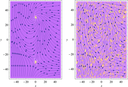
Figure 1. Left: polarization field  and total energy distribution at T = 0 for a vortex–antivortex pair located at
  . Brighter regions characterize larger energy density, where vortices or vortex–antivortex pairs are located. The angle between the axis of the large vortex–antivortex pair and the asymptotic uniform polarization is chosen to be
  . Right: configuration at temperatures close to
  , where a large number of thermally excited small vortex–antivortex pairs strongly alters the power law of attraction in the given vortex–antivortex pair at
  .
.
Download figure:
Standard image High-resolution imageIn dimensionless form, the hydrodynamic free energy functional (playing the role of the hydrodynamic 'Hamiltonian' of the system) is

The short-ranged term  generally reads (
 ) [38]:
where  are constants, and
  is a 'contact interaction' coupling. The 'elastic' constants
  determine the ground-state spin structure, which for
  becomes ferromagnetic. For concreteness, we set
  as the unit of energy, and
  , as well as put
  , choosing as our unit of length the vortex core size (an ultraviolet cutoff). This does not affect our results on the nature of the phase transition (also see the remark after equation (4)). Note that in the hydrodynamic expression equation (4), the constants
  in equation (2) only affect the ultraviolet cutoff, which is irrelevant for the nature of the phase transition; the same applies to the coupling g in equation (2).
The dipolar interaction energy functional entering the hydrodynamic free energy in equation (1) is given by [6, 7, 10]

Here  is the density of polarization charges, and
  represents the dipole–dipole interaction coupling constant. In appendix
We first undertake a qualitative consideration of the scaling behavior of the contributions to the hydrodynamic free energy functional of the planar dipolar XY model for a single vortex–antivortex pair. Note that as in superfluids (see [39], for example), the energy  increases approximately proportional to
  . Therefore the existence of vortices with
  at low temperatures is energetically disfavored. Focusing our attention on the regime
  , we have, typically, that the vortex–antivortex pair size
  . For these vortex–antivortex pairs, using that
  and hence
  ,
,  . Therefore, the energy of a vortex–antivortex pair with
  increases linearly with their size, and vortex and antivortex attract each other with a constant force [8, 10], in sharp distinction to contact interactions, where the force decreases as the inverse of the vortex–antivortex pair size.
For contact interactions, it is well established that the total free energy of the system can be written in the form of a double sum  , where N is the number of vortex–antivortex pairs)

where, in the purely contact interaction case,  , with α is a constant, and
  are the topological charges of the vortices [4, 5] located at
  ,
,  .
.
On the other hand, when strong dipolar interactions come into play, which lead to long-ranged and anisotropic forces in the planar dipolar XY model, the validity of the pairwise summation formula equation (4) is, in distinction to the contact interaction case, highly nontrivial and needs to be thoroughly justified. Because equation (4) is at the heart of our analytical description in terms of plasma physics (see below), we have therefore set up the corresponding Langevin Dynamics simulations and ran extensive checks to establish the validity of equation (4) (see for a detailed discussion of the numerical procedure appendix
We find that the function

describes very well the energy of a vortex–antivortex pair system in the dipolar gas
6
. The quantity  is the 'vortex–antivortex pair tension' coefficient, depending on the coupling strength
  . The logarithmic contribution in
  arises from
  in equation (2) and describes the interaction of vortices in the limit of
  [3–5]. The same numerical calculations also let us establish the functional dependence of
  , which is presented in the inset to figure 2 below. We observe a saturation in the increase of
  with
with  , an effect explained in detail in appendix
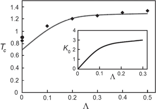
Figure 2. Transition temperature  versus dipole–dipole interaction coupling strength
  computed using equation (16) (dashed line), and numerical result for
  (diamonds). The BKT result [40, 41], corresponding to
  , is shown by a full circle on the
  axis. In the inset the saturation effect for the vortex–antivortex pair tension coefficient
  with increasing dipole–dipole interaction strength
  is displayed. The functional dependence
  forms the input for the evaluation in equation (16) of the critical temperature
  .
.
Download figure:
Standard image High-resolution image3. Plasma analogy
The 'potential'  in (4) is introduced in analogy with the electrostatics of charges:

Here,  ,
,  , and the vortex topological charge density
  .
.
By its definition, the potential  satisfies a Poisson type equation,
  . Here the linear operator
  is defined such that
  , which in Fourier representation reads
 ![${{L}_{{\boldsymbol{k}}}}=1/{{F}_{{\boldsymbol{k}}}}={{\left\{ 2\pi {{K}_{0}}{{k}^{-3}}+4{{\pi }^{2}}\alpha /\left[ {{k}^{2}}\left( k+\alpha \right) \right] \right\}}^{-1}}$](https://content.cld.iop.org/journals/1367-2630/16/5/053011/revision1/njp493738ieqn86.gif) . Let us follow the electrostatic analogy further. Since the energy of a charge (vortex) q placed in the external potential
. Let us follow the electrostatic analogy further. Since the energy of a charge (vortex) q placed in the external potential  is
is  the force, acting on the charge (vortex) is
  , where the quasi-electric field vector
  , the mean field at the charge location. The energy of the pair in this field is

Here the topological dipole moment of a pair is introduced according to  , where
  . The density of the topological polarization charges is

where

is the polarization vector of the vortex–antivortex pair gas, and  is the surface density of vortex–antivortex pairs;
  denotes statistical averaging. After averaging the polarization topological charge inside a contour C,
  , becomes a fractional number in general, while before averaging it must be integer.
The equation for the potential of a point charge Q placed at the origin is  is
is  , where
  . In the weak-field approximation (whose validity we explain in detail in appendix
  of equation (10), we obtain a general formula for
  :
:

Here  is a general nonlocal kernel in an isotropic and translationally invariant medium, connecting electric field and polarization [38]. Hence
  , where
 . Our aim is to describe large-scale effects in a slowly varying field
  corresponding to large r and small k. Henceforth, we can thus take
  , where
  . This approximation holds when the kernel
  decays fast enough with r, such that
  converges. The physical reason behind the latter assumption is that small pairs are far from dissociation and, thus, the vortex–antivortex pair gas at any moment can be approximately subdivided into separated vortex–antivortex pairs. In this approximation the polarization vector is given by (9), where the mean dipole moment of a pair
  is calculated with the help of a Boltzmann type formula with potential energy (7). It is clear from this qualitative consideration that the characteristic length of
  should be of order of the typical small pair dimension,
  : the mean size of a typical small pair with unscreened interaction energy
  is given by
  . Here, we defined thermal averages of moments of the radial distance as follows
where  ,
,  . At
. At  , all parameters approach unity (in our units), therefore
  as well. Note that close to the phase transition this length scale is comparable with the other typical scale of our problem,
  , therefore there is only one characteristic scale at short distances close to
  . So, for the slowly varying field

Therefore χ is the susceptibility of the vortex–antivortex pair gas. Putting everything together, we have for the potential

We define the distance scale

which involves the vortex–antivortex pair tension  and the susceptibility χ of the vortex–antivortex pair gas. At large distances,
  , the dominant contribution to the integral comes from small values of k, for which the
  term in the denominator is negligible. Therefore, since
  , the potential of the 'charge' at large distances is logarithmic:
  , where the constant
  . In the opposite limit,
  , the potential is linear:
  . We propose a simple interpolating expression:
  , so that the energy of a sufficiently large pair of size R is given by

The distance scale  in equation (14) represents an analogue of the Debye shielding radius for 2D interactions of topological charges. We refer the reader for further details on the properties of the distance scale
  to appendix
4. The transition temperature
The standard calculation procedure of the transition temperature for a gas of polarizable vortex–antivortex pairs with interaction (15) gives the following implicit equation for the transition temperature in terms of the susceptibility [3–5],  . At the transition temperature,
  , vortex–antivortex pairs begin to dissociate. This implies that at
  only a small fraction of the pairs is large and close to dissociation. For this reason it is possible to neglect the interactions between the largest vortex–antivortex pairs and calculate the energy of a single large pair approaching its dissociation limit, which is permeated by a cloud of comparatively small bound vortex–antivortex pairs. Hereinafter we will subdivide vortex–antivortex pairs into two classes: small pairs and large, close to dissociation, pairs. The shielding effect arises due to the polarization cloud provided by small pairs, influencing the potential energy of a large pair.
Let us calculate first the polarizability  of a single small pair. The energy of a small pair in an external field
  equals
  . The average dipole moment of the small pair and the susceptibility of the vortex–antivortex pairs gas within the framework of the weak-field approximation (cf appendix
 . Here,
  is the small pair polarizability we are looking for, where we used the definition equation (11). The potential energy of a small pair in the field of the charge Q,
  , approximately does not depend on the position of the pair,
  , so that
  can be considered as a constant.
The surface density of vortex–antivortex pairs,  , at
, at  can be calculated as follows. At
  the vortex–antivortex pairs only start to dissociate and the fraction of large pairs is small. The typical pair is small, and the interaction
  between its vortices is still unscreened. Then, we conclude from basic arguments of statistical mechanics that the partition function of N pairs on a surface with area A is given by
  , using Stirling's formula, and where
 ![${{z}_{1}}=\mathop{\int }^{}{{\text{d}}^{2}}{{r}_{1}}{{\text{d}}^{2}}{{r}_{2}}\exp \left[ -u\left( |{{\boldsymbol{r}}_{1}}-{{\boldsymbol{r}}_{2}}| \right)/T \right]=A{{J}_{0}}$](https://content.cld.iop.org/journals/1367-2630/16/5/053011/revision1/njp493738ieqn149.gif) , which again employs equation (11). Minimization of the free energy
, which again employs equation (11). Minimization of the free energy  gives
gives  ,
,  . Using this result and the relation
  , there follows
  , leading to an implicit equation for the critical temperature

Next we compare the semianalytical solution for  from (16) with the results of the numerical calculation, cf figure 2. As described in detail in appendix
  in a series of simulations with increasingly larger realizations of the model system. In the non-dipolar case,
  (or
(or  ), the equation (16) yields
  . From our numerical calculations, we found that
  . At large
  the transition temperature tends to the constant value
  . From (16) we derive
  . Note that the RG arguments of [10] gave the much larger prediction
  . This in turn implies that it is rather difficult to account for all essential Feynman graphs in order to adequately describe the shielding effect in a RG calculation (which in fact applies equally well to the short-range case
  ).
).
We note that the equation (16) is based on the assumption of the noninteracting small pairs. Rigorously, though, as  , this fails around
  . Hence we expect this approximation to give only an order of magnitude estimate for the susceptibility χ, and the equality sign in equation (16) is to be replaced in that rigorous sense by an ≈. On the other hand, we find from our numerical calculations that the approximation leading to equation (16) still proves to be rather reliable for a sufficiently accurate prediction of the critical temperature, cf figure 2.
5. Conclusion
We have demonstrated both numerically and analytically using an analogy to plasma physics, that vortex–antivortex pairs in the 2D dipolar XY-model dissociate at a critical temperature in a manner familiar from the BKT transition. This is due to the dipole–interaction-induced linear confinement potential in an isolated large vortex–antivortex pair being shielded by a gas of small pairs, in which the large pair becomes immersed around the transition point. Therefore, the logarithmic attraction between vortices in large pairs is restored. By obtaining a physically transparent scenario, we have therefore provided an unambiguous proof that the BKT mechanism is applicable to a much broader class of systems than hitherto established. Our simulations, combined with the analytical approach presented above, give a rigorous confirmation of the qualitative assumptions discussed in [42]. Shielding of the linear interaction in a vortex–antivortex pair implies that the dipole interaction term  is irrelevant (in the sense of the RG), and that the 2D dipolar XY-model belongs to the same universality class as the contact interaction BKT-model corresponding to
  . This conclusion is confirmed in appendix
We finally stress that the planar dipolar XY model (1) fundamentally differs from the commonly studied 2D system with all dipoles oriented perpendicular to the plane
7
, cf e.g., [43], which is a scalar model. Also, it differs from a 'purely' dipolar model (see [24], for example), whose Hamiltonian does not contain the short-range (gradient) term,  , in equation (1). Therefore, the physics behind these models is fundamentally different from the dipolar XY case. For example, the ground state for square lattice in [24] is antiferroelectric, but we have a ferroelectric ground state.
Acknowledgments
The work of AYuV, AET, LIM, and POF was supported by Quantum Pharmaceuticals. The research of URF was supported by the NRF of Korea, Grant Nos. 2010-0013103 and 2011-0029541.
Appendix A.: On the microscopic derivation of the hydrodynamic Hamiltonian
We briefly outline in what follows the derivation of the Hamiltonian equation (1), underlying our analysis, from microscopics. The interaction energy of  polar molecules with dipole moments
  , where
  , equals

where  are the spatial indices,
  , and
, and  . Here
  describes the long-range interaction of molecules
  ,
,  . The function
  represents the short-range part, for example the hydrogen bond interaction in the case of water molecules. In the continuum approximation of hydrodynamics, when the polarization vector,
  , is considered as a slowly varying function, the latter replaces
  , and the summation over molecules
  is replaced by an integration
  , where
  is the moment density and D the spatial dimension. The hydrodynamic approximation is capable to describe the long-range effects which are considered in our paper. After an integration by parts, the long-range part
  takes the form of equation (3).
In the short-range term, we can take  , and the energy density is expanded in ρ. Writing

we use the following definitions and expansions


The tensor  depends only on the distance vector
  . Due to space isotropy it should have the same form in any Cartesian frame, therefore

After integration over  , the nonvanishing contributions contain even powers of
  only. Finally, identifying
  (assuming that all
  have the magnitude μ), the integration
  reproduces the bilinear terms in equation (2).
The quartic 'self-interaction' term,  , stems from a spin saturation effect,
  for large moment densities
  . This saturation can be explained, for example, by the Langevin formula
 ![$s=L\left[ \frac{\mu {{E}_{d}}}{{{k}_{B}}T} \right]$](https://content.cld.iop.org/journals/1367-2630/16/5/053011/revision1/njp493738ieqn202.gif) , with the Langevin function
, with the Langevin function  , yielding
  for a large polarizing electric field
  .
.
Appendix B.: Physical meaning of the distance scale 

The polarization topological charge density of the vortex–antivortex pair gas close to a single topological charge Q equals:  . We conclude that the total charge inside a circle of radius r is given by
  . From this qualitative consideration we thus come to an important conclusion: the charge is essentially shielded,
  , which occurs at a distance scale
  . Close to the phase transition
  . The polarization of the vortex–antivortex pair gas inhibits the linear attraction within large vortex–antivortex pairs which would prevail with shielding not taken into account. Hence we are led to conclude that the phase transition associated with the dissociation of pairs is qualitatively very similar to the BKT transition in a system with
  .
.
Starting from the order of magnitude estimate above, we now consider a more rigorous approach. According to (4) two unshielded, probe charges at a distance r interact as  (in the presented qualitative consideration we neglect the logarithmic term in
  ), where
  is the topological potential of the charge
  . Similarly, for the point charge Q placed at the origin and the probe charge q:
  , where
  . From here and equations (8), (12), we conclude

This yields a differential equation for  :
:

Its solution is given by

This total charge monotonically diminishes with r from  at r = 0 to Q = 0 at
  . From the formula above for the effective charge shielding we again conclude that its characteristic scale is
  .
.
Appendix C.: Accuracy of the weak-field approximation
We verify in this part of the appendix the applicability of the weak-field approximation. Using equation (15), the average interaction between the vortices at finite temperature is ![$\left\langle U\left( R \right)\right\rangle =z_{P}^{-1}\mathop{\int }^{}_{0}^{\infty }\text{d}R\;U\left( R \right)g\left( R \right)={{T}_{c}}\left( 1-4\tau \right)/\left[ \left( -\tau \right)\left( 1-2\tau \right) \right]$](https://content.cld.iop.org/journals/1367-2630/16/5/053011/revision1/njp493738ieqn223.gif) , where
, where  ,
, ![$g(R)=R\exp [-U(R)/T]$](https://content.cld.iop.org/journals/1367-2630/16/5/053011/revision1/njp493738ieqn225.gif) , and the relative temperature
, and the relative temperature  . On the other hand, the typical size of a close to dissociation large pair,
  , can be estimated from the relation
  . Therefore, next to the phase transition,
  , the dimension of a dissociated pair is large,
  , and its topological 'electric' field is small,
  . A condition for the applicability of the weak-field approximation is therefore the existence of a small parameter
  , representing the ratio of the typical topological 'electric' field of large pair,
  to the field inside a small pair,
  .
.
At  , the dissociating pair is so (exponentially) large, that most of the small pairs inside the large pair are far away from the vortex sources of the field such that the field created by these sources is small. Therefore, the weak-field approximation is applicable close to the transition temperature.
Appendix D.: Numerics
We studied the thermodynamics of our model using Langevin Dynamics [44]. Using a discretized representation of the Hamiltonian at every grid point  , we performed a fixed temperature run of sufficient length to get reliable averages. The calculations were performed using periodic boundary conditions on square lattices L×L with the number of independent nodes
  . The Langevin Dynamics dynamical equations are given by:

where γ is a constant that determines the time scale of relaxation. The stochastic thermal noise terms satisfy  and
and  . In the Langevin Dynamics simulations we use a second-order Runge–Kutta algorithm. The equations of motion above are integrated numerically with the sufficiently small discrete time step
  . To compute the dipole–dipole interaction term in equation (2) in an efficient
  way we used a NumPy FFTW realization [45].
The software was first used to check the assumptions leading to equation (4). First we consider the case of zero temperature, T = 0, and checked the additivity rule expressed in (3) numerically by using an imaginary time relaxation method, which is capable to find local minima of the free energy functional on a configuration space of 2D vectors  taken in nodes of a dense square lattice. Following [46], the initial approximation was specified by the complex-valued skyrmion type expression
  , with
  and
and 
 . For a gas of pairs the total charge vanishes,
  . Therefore,
  at
at  , which agrees with the physical boundary condition
  at
at  . At the first stage of imaginary time propagation the cores of the vortex–antivortex pairs begin very slowly to approach which, finally, leads to their annihilation. Due to this mutual attraction, the vortex–antivortex pair therefore is not a real local minimum. Any initial configuration inevitably transfers at T = 0 to the absolute ground state
  . To stabilize vortex–antivortex pairs, 'pinning' of vortices was used by adding to the free energy a term
 ![${{G}_{\text{pin}}}={{\mathop{\sum }^{}}_{j}}{{G}_{j}},{{G}_{j}}=\mathop{\int }^{}\text{d}f{{V}_{j}}(\boldsymbol{r}){{\left[ \boldsymbol{s}(\boldsymbol{r})-{{\boldsymbol{s}}_{0}}(\boldsymbol{r}) \right]}^{2}}$](https://content.cld.iop.org/journals/1367-2630/16/5/053011/revision1/njp493738ieqn253.gif) , where
, where ![${{V}_{j}}(\boldsymbol{r})={{V}_{0}}\exp \left[ -{{\left( \boldsymbol{r}-{{\boldsymbol{r}}_{j}} \right)}^{2}}/{{a}^{2}} \right]$](https://content.cld.iop.org/journals/1367-2630/16/5/053011/revision1/njp493738ieqn254.gif) ,
,  . We investigated multiple configurations with different numbers of vortex–antivortex pairs using the expression in equation (4), and reproduced numerically the total energy within a small error, less than
  (examples of typical distributions are presented in figure D1). The string tension constant
  was calculated by analyzing the mutual forces which prevail in a vortex–antivortex pair by calculating averages of the derivatives of the pinning potential with respect to the positions of the vortices. The accuracy we were able to achieve is limited by the perturbations introduced by the pinning potential, and is sufficient to prove the reliability of the additivity rule equation (4), also cf figure D1. We found that at
  , corresponding to
  , a physical instability of the single vortex–antivortex pair configuration arises: a new small vortex–antivortex pair is spontaneously created in the center of a large vortex–antivortex pair. With further increase of
  , the 'parent' vortices are immersed into a cloud of small polarized vortex–antivortex pairs, i.e. dipoles with zero total topological charge. Polarization of vortex–antivortex pairs leads to a net topological charge density (cf the discussion after equation (9)) and, hence, to a reduced increase of the line tension
  with
with  . Ultimately, this leads to a saturation effect:
  at
at  (see the inset of figure 2). The spontaneous creation of pairs follows also from the expression (4): at
  the energy of the large (
 ) pair decreases with the emergence of a new small pair in the center. This occurs at
  , if we choose
  /
/ .
.
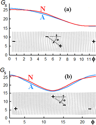
Figure D1. Free energy of a uniformly polarized 2D spin system with a small vortex–antivortex pair in the center of a large pair (a) and for a slightly shifted small pair (b) versus the angle (in units  ) between the axis of the small pair and the x axis. Red (N) and blue (A) curves correspond to the numerical calculation and the analytical approximation in equation (3), respectively;
  .
.
Download figure:
Standard image High-resolution imageTo explore the critical behavior of the model depending on the dipole–dipole interaction coupling constant  numerically we use Binder's method [47] and calculate the parameter
  ('Binder's cumulant') versus temperature. Here
  ,
,  and the statistical averaging is done in a manner equivalent to the average over polarization configurations obtained with Langevin Dynamics. The intersection point of Binder's cumulants for different values of the system size L gives
  , as shown in figure D2. In the symmetric phase,
  ,
,  as
as  , where A is the surface area. In the symmetry-broken phase,
  ,
,  . At the critical point,
  tends towards a universal value
  , which is specific for each model, and is determined by its universality class [47, 48]. To determine the universality class of the model at hand it seems natural to simply compare our value
  with that for the pure BKT-model without dipole–dipole interaction. According to detailed numerical results [49, 50], the magnitude of
  does not depend on the simulation details, but, in fact, the value
  itself '...depends sensitively on boundary conditions, details of the clusters used in calculating the cumulant, and symmetry of the interactions or, here, lattice structure...,' quoting [49]. As a consequence, we have to compare our result with others under the same conditions. We know two such results for
  :
:  for the XY-model [49], and
  for the generalized XY-model [51]. As for the present dipolar XY-model, one has
  in a wide range of
  values [19, 20].
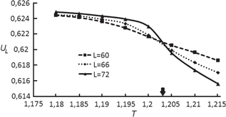
Figure D2. Explanation of Binder's approach to obtain the critical temperature [47]. Binder's parameter  was calculated for
  ; the intersection point for different lattice sizes L yields
  (indicated by the bold arrow).
Download figure:
Standard image High-resolution imageFootnotes
- 6
The function
contains logarithmic and linear terms at arising from and , respectively. At vortices annihilate, therefore . At the linear behavior of is imposed by two nearby topological charges, which stems from . The chosen form of accounts for these features. - 7
The bulk charge density of dipoles oriented perpendicular to the plane, residing inside a homogeneous layer of thickness H,
, equals ; however, the surface charge density vanishes. This implies that long-range effects, which are determined by , are absent.


