


Abstract
The decay of temperature of a force-free granular gas in the homogeneous cooling state depends on the specific model for particle interaction. For the case of rough spheres, in recent experimental and theoretical work, the coefficient of restitution was characterized as a fluctuating quantity. We show that for such particles, the decay of temperature with time follows the law  which deviates from Haff's law, T ∼ t−2, obtained for gases of particles interacting via a constant coefficient of restitution also from
  obtained for gases of viscoelastic particles. Our results are obtained from kinetic theory and are in very good agreement with Monte Carlo simulations.
Export citation and abstract BibTeX RIS

Content from this work may be used under the terms of the Creative Commons Attribution 3.0 licence. Any further distribution of this work must maintain attribution to the author(s) and the title of the work, journal citation and DOI.
1. Introduction
Granular gases, that is, ensembles of dissipatively interacting macroscopic particles may be considered as a model for granular matter in the dilute limit. The dynamics of granular gases is characterized by ballistic trajectories of the particles, interrupted by instantaneous dissipative collisions. In physical terms, the duration of collisions are considered negligible as compared with the time of mean free flight. This paradigm may serve as a definition of the term 'granular gas' in contrast to other granular systems where the particles may interact via permanent or long-lasting contacts. Besides of its practical importance for the description of natural phenomena, such as clouds of dust or the rings of the large planets of our solar system, granular gases have been intensively studied for their rich phenomenology.
From the point of view of theoretical physics, of particular interest is force-free granular gas, that is, an spacially infinite system in the absence of external gravity and boundaries due to confinement. For such systems, statistical physics provides powerful tools like the Liouville- and Boltzmann equation which may be adopted to account also for dissipative particle interactions [3, 4]. Subsequently, the full hydrodynamics can be derived, including the corresponding transport coefficients, e.g. by exploiting the Chapman–Enskog approach [4–6].
Because of the dissipative nature of particle interaction, granular gases are always in non-equilibrium, giving rise to many interesting phenomena, such as non-Maxwellian velocity distribution, e.g. [7], correlations of the velocities, e.g. [8], anomalous diffusion [9] and finally the instability of the homogeneous state in the long-time evolution [10] which may be transient, depending on the details of the particle interaction [11].
Starting from a homogeneous state at the time of initialization the evolution of a granular gas follows certain stages: (a) in a fast first stage, the distribution function of the gas rapidly converges to its native velocity distribution: on a time scale corresponding to a few collisions per particle, the distribution looses memory of the initial distribution and becomes essentially near Maxwellian, except in the high speed tail, where convergence is much slower [12] (mathematically it takes infinite time). (b) In the second stage of its evolution, the granular gas stays homogeneous, while the absolute velocity of the particles decays in time which may be expressed by a decay of temperature [13]. Therefore, this stage is called homogeneous cooling state (HCS). The velocity distribution and in particular temperature (its second moment), describe the HCS exhaustively, that is, the time dependence of the one-particle distribution function is solely a function of temperature. The distribution differs from the Maxwellian in two main points: the main part of the distribution, that is for v ∼ vT , where vT is the thermal velocity, is distorted which may be described by a low-order Sonine expansion [14]. For large velocities, v ≫ vT , the distribution reveals an overpopulated high-energy tail,  [7, 15] in difference to
  expected for molecular gases. The high-energy tail was found first from kinetic arguments [15] and numerical simulations and later from a high-order Sonine expansion [16]. The properties of granular gases in the HCS have been very intensively studied, e.g. [7, 17, 18], revealing in particular the breaking of equipartition in frictional [19, 20] or polydisperse [21–24] granular gases. The HCS has also been employed in derivations of Green–Kubo relations for granular gases [25, 26]. (c) The third stage of the evolution is characterized by the instability of the HCS and the formation of dense clusters, due to localized fluctuations of the density, associated with the instability of the shear mode [10, 27], for large enough systems [10, 27–29]. Those fluctuations, by locally modifying the collisions frequency (and thus energy dissipation), break the pressure balance and generate a positive feedback [10]. (d) Depending on the details of particle interaction, the cluster state may become unstable [11] because for small impact velocity, defined as the component of the relative velocity of two colliding particles along the direction joining their center, the collisions become less and less dissipative expressed by the coefficient of restitution approaching unity. In this case, the clusters resolve and the granular gas turns back to a homogeneous state at very low temperature. Resolution of the clusters may be observed for gases of viscoelastic spheres [11] as well as for charged particles and similar cases [30–32].
Whether the stages of the evolution of a granular gas occur on separate time scales depends mainly on the extend of energy loss due to dissipative collisions, expressed by the coefficients of restitution. In this paper we assume that the dissipation is small enough such that the HCS (stage (b)) exists for a certain time interval. That is, we assume that there exists an interval in time where the temperature is the only system characteristics which varies in time, before at stage (c) correlations of density and velocity become important.
Apart from particle number density and initial temperature, the key parameter, characterizing the kinetics of granular gases is the coefficient of restitution, ε, quantifying the loss of energy of the relative particle velocity due to collisions. While in most references it is assumed that ε is a material constant, detailed analysis of the collision process as well as experiments show clearly that the coefficient depends on the impact velocity which was mentioned in the literature already long ago, e.g. [33–36]. Moreover, even for virtually perfect spheres like ball bearings, in experimental measurements one observes significant scatter because of microscopic surface asperities [37–40]. This scatter may be expressed by considering the coefficient of restitution as a fluctuating quantity. The aim of this paper is to address the question how the stochastic nature of dissipative particle interactions influences the decay of temperature of a force-free granular gas as a function of time.
Throughout this paper we assume that the particle size and material properties as well as the thermal velocity and the number density of the gas are chosen such that the dynamics can be described by a purely repulsive coefficient of restitution. In particular, we require that the characteristic impact velocity is large enough to neglect van der Waals cohesive forces and small enough to avoid plastic deformation and brittle of the particles.
The structure of the paper is as follows. In section 2, some general results concerning the decay of temperature in the HCS are discussed. Section 3 presents a numerical and analytical analysis of the temperature behavior in the case of a stochastic, velocity-dependent coefficient of restitution. Section 4 is devoted to the study of the velocity distribution function, employing a slightly simplified (Laplacian) distribution for the coefficient of restitution. Finally, some conclusions are presented in section 5.
2. Decay of temperature in the homogeneous cooling state
2.1. Constant coefficient of restitution and Haff's law
The inelasticity of a collision between two particles may be characterized by the coefficient of restitution, ε, relating the normal component of the particles' relative pre-collisional velocity, v'ij ≡ v'i − v'j, whose norm defines the impact velocity, to that of the post-collisional relative velocity, vij,

where

 ,
,  are the pre-collisional velocities,
  ,
,  are the post-collisional velocities, and

is the unit vector at the instant of contact. Using these definitions we obtain the post-collisional velocities via

Because of the dissipative nature of the collisions, characterized by ε < 1, the absolute velocities of the particles decay on average, which may be expressed by a decay of temperature. If we define temperature in analogy with the temperature of molecular gases,

where m denotes the mass of a particle, and an overline denotes an average over the particles, the evolution of temperature is given by

where n and d are the number density of the gas and the diameter of the particles, respectively. If the coefficient of restitution is assumed independent of the impact velocity, ε = const, we obtain Haff's law [13],

where T0 is the initial temperature, that is asymptotically T(t) ∼ t−2. Haff's law is the most simple expression for granular cooling. The asymptotic form has been confirmed experimentally, where gravity was compensated by diamagnetic levitation [41]. Note that Haff's law is valid after the relaxation of the initial (Maxwell-) distribution to the native distribution; during this very short relaxation, the cooling is dominated by exponential terms [42]. Haff's law seems to be rather general; it was shown to hold true for smooth spheres in dimension 2–6 [43] as well as for a gas of needles [44]. Even beyond the HCS, that is at later times when significant correlations emerge, Haff's law is a fair approximation [18].
Somewhat unclear is the influence of the shape of the particles on the cooling law. While Haff cooling is observed for needles in 2d [44] and ellipsoids in 3d [45], in simulations of 'elongated' sharp edged particles T ∼ t−5/3 was found [46].
2.2. Temperature decay due to an impact-velocity dependent coefficient of restitution
While the assumption ε = const simplifies the kinetic theory significantly, for realistic particles, the coefficient of restitution is a function of the impact velocity, ε = ε(v). For non-adhesive viscoelastic spheres, ε(v) can be obtained by integrating Newton's equation of motion describing the dynamics of the collision when the (normal component of the) interaction force is given by a generalized Hertz law [47]:

where  is the compression of the colliding spheres (
  and
and  denoting their positions), Y is the Young modulus, νp is the Poisson ratio and the dissipative constant A is a function of the elastic and viscous parameters. The coefficient of restitution is then given by
  , where tc is the duration of the collision, determined by requiring
  . This complicated problem was solved rigourously [48] with the solution
hi being analytically known, universal constants. For realistic materials, equation (8) agrees well with experiments, e.g. [49], while a constant coefficient of restitution disagrees even with a dimension analysis [50]. From equation (8) follows that ε depends on the temperature in equation (6). In this case, the temperature decays due to

with the solution

that is, asymptotically T(t) ∼ t−5/3.
In many cases, temperature decays algebraically with time, but this is not always the case: for ε due to

temperature decays logarithmically slow [31]:

where κ = const. The same behavior was found for particles with long range (electrostatic) repulsive interaction [30–32] while for attractive long range interaction enhanced cooling (compared with Haff's law) was reported [32].
Note that for the derivation of equations (7), (10) and (12) it was assumed that the state of the system is described by the second moment of the velocity distribution. In general, however, due to the non-Maxwellian distribution, the kinetic state depends also on higher (even) moments [51, 52], that is,

For the cases discussed above, it was shown [53, 54] that the deviations of the distribution function from the Maxwellian, expressed by the Sonine coefficients, changes the decay rate, τ and τ', but not the functional form of the function T(t). The other type of deviation from the Maxwellian, that is, the overpopulated high-energy tail [15] leaves also its fingerprints in the temperature decay law, but its effect is very small [12].
2.3. Decay of temperature beyond the homogeneous cooling state
When the system left the HCS due to the formation of correlations in the velocity field and cluster formation, Haff's law is invalidated. Most references on the cluster state describe slower cooling compared to Haff's law, e.g. [18]. Also Dominguez and Zenit [55] describe cooling according to T(t) ∼ t−k with  , depending on the volume fraction. Asymptotically, for large time the temperature decays as T ∼ t−1 [56].
3. Decay of temperature for fluctuating coefficient of restitution
3.1. Stochastic coefficient of restitution
Realistic granular particles are certainly not perfect spheres. Even nearly spherical particles like glass spheres or precision steel spheres as used in ball-bearings, reveal surface asperities. These asperities lead to a surface roughness and in turn to a stochastic behavior of the particles in collisions which may be expressed by a stochastic coefficient of restitution. Even for microscopically small asperities, it was shown that the fluctuations of the coefficient of restitution are significant [40]. Based on experiments consisting of 2 × 10⁶ single impacts, performed by means of a robot [40] it was found that the functional form of the stochastic coefficient of restitution is strongly non-Gaussian. Instead, its probability distribution is Laplace-like, that is, composed of two exponential functions. Notably, the fluctuations observed in experiments exhibited a remarkable asymmetry:
where εmax(v) is the value of ε where ρv(ε) adopts its maximal value. It was found that the function εmax(v) is the same as for viscoelastic spheres, equation (8).
The probability distribution, equation (14), was experimentally found and confirmed by simulations where the surface roughness was modeled by a large number (∼ 106) of microscopic spheres covering the surface of the sphere [40]. Figure 1 is obtained from experimental data [40] where the coefficient of restitution of a particle in contact with a flat plate is investigated as a function of the impact velocity. It shows the normalized frequency ρ(ε) of measurements of a certain value of ε for several small intervals of the impact velocity v.
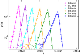
Figure 1. Histograms of the coefficient of normal restitution for impact velocities from small intervals. Each histogram represents a certain impact velocity. The lines are exponential fits.
Download figure:
Standard image High-resolution imageThe mathematical form of equation (14) is a Laplace-probability density

with two generalizations:
- (a)The mean value
 is replaced by a decaying function of the impact velocity, εmax(v), to account for the physical fact that the coefficient of restitution increases with decreasing impact velocity. This behavior is well known for dry viscoelastic particles and for impact velocity small enough to avoid plastic deformations and large enough to neglect surface effects like adhesion, e.g. [57, 58].
 - (b)The Laplace distribution, equation (15), is symmetric with respect to, while the distribution density, equation (14) is asymmetric, characterized by two (impact velocity dependent) standard deviations σp(v) and σm(v), for ε > εmax and ε < εmax, respectively. The asymmetry can be explained considering the mechanism of energy transfer between the (external) linear degree of freedom and internal degrees of freedom during the collision [40]. Due to this asymmetry, strictly speaking, the maximum of the distribution function, εmax(v) is different from the expectation value , however, both values are very close.


In the subsequent analytical and numerical calculations we will assume that the coefficient of restitution obeys the probability density function equation (14).
Fluctuating coefficients of restitution were also introduced in other contexts such as to model heating through collisions in a vertically vibrating granular system [59, 60], to describe a gas of one-dimensional particles accounting for internal degrees of freedom [61, 62] and in gases on Maxwellian molecules [63] to investigate the high velocity tail of the distribution function. More general random collision rules were considered in [64]. All these models are rather different from our collision model, equation (14), in that the functional form of the coefficient of restitution was not based on considerations of the physical processes during collisions.
3.2. Decay of temperature—kinetic theory
At the kinetic level, the system is described by a distribution function for the velocities,  , by mean of which one can express the number density field, and temperature, as


The equation of motion for T is given by

where γ is the cooling coefficient, describing the rate of decay of the kinetic energy (multiplied by  ), due to the inelasticity of the collisions. Using the velocity transformations, equation (4), the change of energy ΔE in a collision between particles with velocities
  and
and  , along the direction spanned by the unit vector
  , and characterized by a coefficient of restitution ε, is given by

In addition, the collision frequency ν12 of such collisions is

where d is the diameter of the particles. Therefore, the cooling coefficient is given in terms of the distribution function by

where a factor 1/2 has been included to avoids double counting of collisions,  denote the conditional probability for a coefficient of restitution ε, given a normal relative velocity v, H is the Heaviside step function and the integration range of ε is [ − ∞,+∞]. Note that the distribution function depends on the distribution
  . In order to take into account this dependence, one needs to solve the Boltzmann equation pertaining to the system. For the moment, we will for sake of simplicity neglect this dependence and assume that the deviation of the velocity distribution function from the Maxwell distribution

is small. This assumption is reasonable since the range of interest for the coefficient of restitution is of the region  due to the experimental results on which this paper is based [40], see figure 1. Recall that the value of the second Sonine coefficient (corresponding to the inelastic correction to the Maxwellian distribution, cf section 4) for a granular gas with ε = const is a2 < 0.01 in this region [14, 54]. In section 4 we will consider a slightly simplified distribution
  and show that the deviations from the Maxwellian are small indeed.
If we approximate the distribution function by a Maxwellian,  , the cooling coefficient γ reads

where brackets denote an average over ε. It appears that the evolution of the temperature deviates from the decay corresponding to the case of non-fluctuating coefficient of restitution due both to the variance of the distribution, and to the asymmetry of the distribution function, ρv(ε) (i.e. 〈ε2〉 ≠ ε2max). While the former has negligible effect, the latter has a qualitative influence on the asymptotic evolution of the temperature. By using the coefficients σm(v) and σp(v) obtained from simulation data (cf section 3.3 below), the average coefficient of restitution corresponding to the distribution (14):

is found to be well described by a function of the form

(see figure (2)). A straightforward calculation then yields

i.e. solving equation (18):

that is,

with the constant τρ defined by equation (27). Comparing this result with the decay of temperature of a gas of viscoelastic particles [48, 65],  , equation (10), we obtain that the fluctuating coefficient of restitution lets the gas cool noticeable faster but slower than gases of particles interacting via ε = const, where
  , according to Haff's law [13].
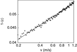
Figure 2. Numerical data (obtained as described in section 3.3) (crosses) and best fit (solid line) for  , plotted as a function of the impact velocity, in logarithmic scale. The data are well described by a function of the form:
  , with δ* = 0.05317, and
  .
.
Download figure:
Standard image High-resolution image3.3. Decay of temperature—numerical simulation
3.3.1. Numerical description of the stochastic coefficient of restitution
For the direct simulation Monte Carlo (DSMC) simulation we need random numbers distributed according to  as given by equation (14) where εmax(v) in turn is given by equation (8). Using the inverse transformation method [66], these random numbers have to be computed from standard random numbers, x, equally distributed in the interval x∈(0,1), available on the computer. The cumulative distribution function

maps each value of ε to a number in the interval (0,1). So if ϱ can be inverted, ϱ−1(x), obeys the distribution ρ if x is an equally distributed random number, x∈(0,1).
For later use, we write the distribution function more general,

where the coefficients a,b,c and d follow from equation (14). Its cumulative distribution function reads
with the inverse
In this way, we obtain random numbers distributed according to ρ(ε) from equidistributed random numbers x∈(0,1).
Note that the functions ϱ−1v depend on the impact velocity through  . To obtain a random number according to ρv(
 ), thus, we first determine
  and then by means of a random number x∈(0,1), via equation (32) we obtain the desired random number. In principle,
  could be computed via equation (8) by truncating the series at a certain order. However, this series in
  converges very slowly [48]. Therefore, we prefer the Padé approximation of order [1/4] provided in [67]

with the universal (material independent) constants c1 = 0.501 086, b1 = 0.501 086, b2 = 1.153 45, b3 = 0.577 977, b4 = 0.532 178.
For demonstration, figure 3 shows a histogram of 106 random numbers obtained by application of the described algorithm. The material constant β = 0.0467 was used, corresponding to the experimental values given by Montaine et al [40] for the collision of stainless steel spheres.
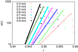
Figure 3. Coefficients of restitution obeying the distribution equation (14), generated using the described algorithm. Each histogram, corresponding to a certain impact velocity, was obtained from 106 values of the coefficient of restitution (β = 0.0467).
Download figure:
Standard image High-resolution image3.3.2. Direct simulation Monte-Carlo details
To study the decay of temperature in the HCS, we apply DSMC [68, 69]. DSMC simulations of dilute granular gases have been first performed by Brey et al [17]. DSMC is by orders of magnitude faster than molecular dynamics (MD) (event-driven as well as force controlled MD), however, its main advantage compared to MD is that DSMC is not a particle simulation [70] but a tool to integrate the Boltzmann (or Boltzmann–Enskog) equation by means of a Monte-Carlo procedure. This allows us to compare the results of a DSMC simulation directly with the results obtained from the kinetic theory. When investigating a granular gas in the HCS, MD is restricted to almost elastic particles,  , and low density, to avoid formation of correlations of different kind, conflicting the homogeneous state. In contrast, DSMC works for all values of the coefficient of restitution and density by avoiding correlations. We wish to remark here that large part of the literature confirms that influence of the correlation of particle velocities due to inelastic collisions on the cooling rate is small, e.g. [71–75], which has, however, also been questioned [76].
In our simulation, at each time step a pair of (quasi-) particles is selected randomly with equal probability. A collision according to the collision rule, equation (4), was executed if

where RND is a uniformly distributed random number from the interval RND∈(0,1) and vT is the thermal velocity. To compute the post-collisional velocities using equation (4) we determined a random unit-vector  . The term 7vT is an estimate for the smallest upper bound of the average normal velocity, see [69] for justification of this term. The simulation was performed with 105 quasi-particles, initialized with a Maxwellian velocity distribution according to the thermal velocity T0 = 1.
3.3.3. Decay of temperatures obtained from DSMC simulations
We simulated a granular gas of particles interacting via a fluctuating coefficient of restitution due to equation (14) in the HCS and computed the granular temperature as a function of time via equation (5). For large times, the temperature decays according to a power law, T ∼ t−k, with the best fit k = 1.71 being in excellent agreement with the result obtained from kinetic theory, equation (28),  . Figure 4 shows the DSMC simulation data with a best fit of the function

with a fit value for τ together with the analytical result, equation (28). The asymptotic decay due to Haff's law [13] (for ε = const) and for a gas of viscoelastic particles [65] is also shown.

Figure 4. Evolution of the granular temperature of a gas of 105 particles interacting via a fluctuating coefficient of restitution. The full line shows the analytical result, equation (28), the symbols show the simulation results. The dashed lines mark the asymptotic behavior for gases of viscoelastic particles,  [65], and particles interacting via a constant coefficient of restitution, Haff's law, T ∼ t−2 [13].
Download figure:
Standard image High-resolution imageThe result deviates from Haff's law (k = 2) [13] as well as from the evolution of temperature for a gas of viscoelastic particles ( ) [65]. Note that the deviation from the case of viscoelastic particles originates from the asymmetry of the probability function, ρv(ε). Although the median of the coefficient of normal restitution equals the expression for viscoelastic spheres [48, 65], the mean value deviates considerably because of the skewness of the functions.
4. Laplace distributed coefficient of restitution
The cooling coefficient γ depends on the distribution ρv(ε) explicitly, as shown by equation (21), but also implicitly, since the velocity distribution function,  , obviously depends on the choice of ρv(ε). In section 3.2, we assumed that the deviation of the distribution function from a Maxwellian is small, based on (a) our numerical observations, section 3.3.3, and (b) the fact that for ε = const the second Sonine coefficient quantifying the deviation of
  from the Maxwell distribution, is very small (
 ) in the range of ε ≈ 0.98 being of interest here. In this section we wish to quantify the claim that the distribution function is close to a Maxwell distribution to—à posteriori—justify the above assumption. In this section we are not interested in the absolute value of the coefficient of restitution (characterized by εmax), nor in the skewness of its distribution, ρv(ε), being both of major importance for the decay of temperature. Instead, here we consider the fluctuations of the coefficient of restitution, ε. To this end, we reduce the full distribution function, equation (14), to the Laplace distribution, equation (15), by neglecting the velocity dependence and the skewness of the distribution. Apart from these details, the Laplace distribution, equation (15), is of the same characteristic shape as equation (14), that is, it consists of two exponentials

The Boltzmann equation describing a granular gas in the HCS at the kinetic level reads, in the case of a velocity-independent (fluctuating) coefficient of restitution:

where  is the (velocity independent) distribution of the coefficient of restitution, and
  is the Boltzmann collision operator corresponding to a fixed coefficient of restitution

The unit vector  , the sets
  ,
,  of the pre- and postcollisional velocities and the relative velocity,
  , were introduced in equations (2)–(4).
In order to take into account the inelastic corrections to the Maxwellian distribution, we consider a normal solution of the Boltzmann equation, i.e. a solution depending on time through its (functional) dependence on the hydrodynamic fields. In the case of a homogeneous system, the only hydrodynamic field which is time dependent is the temperature, and we seek a similarity solution in the time-independent scaled velocity,

that is, we scale the velocity by the thermal velocity to compensate the decay of temperature. While this is the standard procedure in the physical literature, the pure existence of the time-independent similarity solutions is not mathematically proven [77]. Assuming it exists, the Boltzmann equation, equation (37), in this case reduces to

The standard way to solve the above equation is to represent the distribution function,  , in form of a truncated series of Sonine polynomials [78], whose coefficients characterize the deviation of
  from the Maxwell distribution:

where N is the order of truncation, and the Sonine polynomials are defined by [78]
This method was first applied by Goldshtein and Shapiro [14, 54] to granular gases. Note that there are different truncation schemes to compute the Sonine coefficients ai [16, 79–81]. Using the expansion equation (41) in equation (40) and in equation (21) for γ, and projecting back on the Sonine polynomials, one obtains a system of equations for the coefficients  This system is to be solved together with the orthogonality conditions expressed by the requirements equations (16) and (17) that the number density and temperature are given by the appropriate moments of the distribution function. Those conditions impose constraints on the coefficients {ai}. In particular, due to the orthogonality properties of the Sonine polynomials, these requirements imply a0 = 1 and a1 = 0. Truncating the series, equation (41), to the first non-trivial order (N = 2) and assuming that the coefficient a2 is small enough so that orders higher than linear can be neglected, one readily obtains the following expression for the correction:

where brackets denote the average over the values of the coefficients of restitution. In the case of constant ε, the standard expression for a2 is recovered [14, 54, 82]. Using the above expression, together with the expansion (41) in equation (21), the cooling coefficient reads, to linear order in a2

In the case of a Laplace distribution, equation (15), γ is given by
where

corresponds to the correction due to a2 to the cooling coefficient. It can be checked that this correction is negligible (cf figure 5). For standard deviations σ < 0.1, this correction is lower than 4% even for low values of the mean coefficient of restitution, i.e. highly inelastic systems. For the value 〈ε〉 = 0.98 considered here, the correction is lower than 1%. In order to characterize the influence of the fluctuations, the ratio

is plotted in figure 6 as a function of σ, for a mean coefficient of restitution 〈ε〉 = 0.98, together with simulation results for the same quantity, obtained by fitting the cooling curve to Haff's law. Agreement between simulation and theory is excellent, and the fluctuations are seen to have a rather weak influence, yielding a deviation of about 10% with respect to the non-fluctuating case, even in the case of relatively large fluctuations σ = 0.05. (Notice that in this case, the coefficient of restitution can exceed unity at very low probability.)

Figure 5. The correction γ(1) to the cooling coefficient due to a2, as a function of 〈ε〉, for some values of σ. For σ < 0.1, the contribution of a2 to the cooling coefficient is always lower than 4%.
Download figure:
Standard image High-resolution image
Figure 6. Simulation results and analytic expression for the relative difference  between the cooling coefficients of a gas with fixed coefficient of restitution and of a gas with Laplace distributed random coefficient as a function of the standard deviation σ of the distribution, for a mean value of ε = 0.98. The discrepancy is relatively small even for large fluctuation. Simulation and theory are in almost perfect agreement.
Download figure:
Standard image High-resolution image
5. Conclusion
We considered the decay of temperature of a force-free homogeneous granular gas of particles interacting by instantaneous binary collisions, where we took the stochastic nature of particle interaction into account. To this end, we employed the velocity dependent conditional distribution for the coefficient of restitution described recently in [40], based on both large scale experiments and numerical simulations.
By means of kinetic theory we find a novel type of asymptotic decay of temperature following the law  . This function is in contrast to both standard cases of temperature decay in dilute gases of purely repulsively interacting spheres, namely Haff's law T ∼ t−2 corresponding to a gas where the particles interact via a constant coefficient of restitution, and to
  corresponding to a gas of viscoelastic spheres. The result was checked by numerical DSMC simulations and very good agreement was obtained. Although the deviation of the new exponent from the exponent for gases of viscoelastic spheres is rather small, both cases can be clearly distinguished in DSMC simulations. That is, the stochastic nature of particle interaction leaves a clear footprint in the macroscopic properties of the gas.
The deviation of the exponent from the standard cases was shown to be associated with the asymmetry of the distribution function of the fluctuating coefficient of restitution. This asymmetry results in a difference between the (impact velocity dependent) mean value and the (viscoelastic) most probable value of the coefficient of restitution. Despite the obtained qualitative difference in the decay of temperature, the effect is quantitatively small, due to the small variances of the distribution for ε found in simulation and experiments [40].
In order to à posteriori justify the assumption of a Maxwellian velocity distribution employed for the analytical calculation (but not for the DSMC simulations!), we considered a simplified (velocity-independent) probability distribution of the coefficient of restitution of Laplace type. For this case, we solve the Boltzmann equation via a truncated Sonine expansion to obtain the velocity distribution of the gas particles. We could show that the correction to the Maxwellian distribution due to the inelasticity is negligible indeed, justifying the overmentioned assumption.
For non-spherical particles of more complex shape, stronger effects can be expected as a result of a wider distribution of the fluctuating coefficient of restitution.
Acknowledgments
This work was supported by the German Science Foundation (DFG) through the Cluster of Excellence 'Engineering of Advanced Materials'. DS thanks the Humboldt Foundation for support via the Alexander von Humboldt post-doctoral fellowship. We acknowledge support by Deutsche Forschungsgemeinschaft and Friedrich–Alexander–Universität at Erlangen–Nürnberg within the funding programme Open Access Publishing.
Appendix.: Derivation of equation (26)
Substituting equation (22) into equation (23), the cooling coefficient reads

Using the form equation (25) in the above equation, neglecting the variance of  (the latter being of the order of the square of the small standard deviations σm and σp) and quadratic terms in δ* yields

First, the integral over  is readily performed:

Next, upon changing the variables  and
and  to
to
For  , one obtains equation (26).