


Abstract
The dynamics and structure of rotating homogeneous turbulence is investigated through the statistical properties of the 'perceived' velocity gradient tensor, defined by interpolation from the locations and velocities of a set of four particles. The results of direct numerical simulations of forced homogeneous rotating turbulence at different Rossby numbers are presented. We thus provide a multi-scale analysis of the dynamics of rotating turbulence and some of its important features. We present scaling laws for second- and third-order moments of the perceived velocity gradient tensor. We relate the distribution of the enstrophy and strain variance, and of their production terms, to the topology of the flow, thanks to conditional probability density functions. These quantities demonstrate the role played by the Zeman scale in the elementary processes of rotating turbulence, when compared to the scale at which the perceived velocity gradient tensor is measured.
Export citation and abstract BibTeX RIS

Content from this work may be used under the terms of the Creative Commons Attribution-NonCommercial-ShareAlike 3.0 licence. Any further distribution of this work must maintain attribution to the author(s) and the title of the work, journal citation and DOI.
1. Introduction
Particle-laden turbulent flows have recently received considerable attention due to their widespread occurrence in natural and industrial systems. In particular, many efforts have been devoted to the investigation of the dynamics of solid particles in turbulence, with theoretical [1], experimental [2–4] or numerical approaches [5–7]. Objects of small size (in practice, sufficiently smaller than the Kolmogorov scale) and of density equal to that of the carrier fluid are expected to behave like passive tracers. This property has been used for a long time in experiments (particle image velocimetry and particle tracking velocimetry techniques) in order to characterize fluid flows in general. It has also inspired a new approach to turbulence, based on the Lagrangian point of view. For instance, tracking a fluid particle or a pair of such objects naturally brings some insight into turbulent dispersion and mixing.
A more refined description of incompressible flows is given by the Lagrangian dynamics of the velocity gradient tensor, whose components are mab = ∂avb. Many works have been devoted to the modeling of the dynamics of this object along a fluid trajectory, starting from the restricted Euler dynamics [8, 9], and giving a series of increasingly refined models [10–13] (see [14] for a recent review). A model for the dynamics of m in the presence of rotation has recently been proposed and analyzed [15]. Another quantity of interest is the so-called 'perceived velocity gradient tensor', of components Mab, defined by interpolation from the locations and velocities of a set of four tracer particles, called a tetrad [16]. The Lagrangian statistics of this tensor provide some information on the flow topology and have been the object of different investigations: measurements in experiments and in velocity fields coming from direct numerical simulations (DNS) of homogeneous and isotropic turbulence [17, 18], or modeling [16, 19–21] (see [22] for predictions in homogeneous shear turbulence).
In the case of anisotropic turbulence, significant modifications of the dynamics of the turbulent field imply changes in the fluid properties at all scales by symmetry breaking, as in turbulence subject to solid body rotation. The anisotropy of the flow may be observed at the level of one-point statistics, with, for instance, a separation of the rms velocity components, but also considering velocity gradients, thus evidencing the extension of anisotropy throughout all scales, from integral to dissipative ones. The geometrical information provided by tetrads therefore permits us to quantify the detailed structure of the flow, as well as its scale-dependent energetic equilibrium. Rotating turbulence is a heavily investigated topic, due to its relevance in geophysical flows but also in several instances of industrial flows, e.g. in turbomachinery. Even restricted to the very simple configuration of homogeneous flows, the effect of the rotation, mediated by the Coriolis force, on the structure and dynamics of turbulence is still a relevant research topic, since the description of anisotropic turbulence is not yet amenable to theoretical advanced theories such as that of Kolmogorov for isotropic turbulence. Several efforts are thus devoted to the characterization of the anisotropic structure of rotating homogeneous turbulence, by experimental means [23, 24] and DNS [25], to cite but a few recent ones. The statistical modeling of rotating turbulence is often tackled in the very low Rossby number limit that produces wave turbulence, in which inertial waves interact in a weakly nonlinear way among each other (see the recent book by Nazarenko [26] or [27]). These approaches to rotating turbulence demonstrate the presence of three-dimensional vortices elongated along the rotation axis, as a result of anisotropic nonlinear transfer of energy [28] or of the axial propagation of inertial waves [24], depending on the ratios of the turbulent timescale to inertial wave timescale, i.e. the Rossby number  , where u and L are the velocity and integral length scales and
  is the rotation rate. This strong anisotropy propagates throughout all scales when the Zeman scale
  (ε is the dissipation) is smaller than the smallest scale of turbulence [25]. A multiscale characterization of the anisotropy of rotating turbulence thus requires specific statistics, e.g. directional spectra of two-point velocity correlations [28, 29], or velocity increments and structure functions [23, 30, 31]. A third approach is the analysis based on variable scale gradient tensors [16], which we consider in this paper. Its application is original in the framework of rotating turbulence statistics.
One also expects to find traces of the anisotropic Eulerian structure of rotating turbulence on Lagrangian statistics, such as the statistics of one- or two-particle dispersion, with separate scalings in the axial and transverse directions, as observed experimentally [32] or by DNS and stochastic modeling [30, 33]. Among other results, these studies show the subtle relationships between third-order moments of velocity and multi-point correlations along the Lagrangian trajectories.
The paper is organized as follows. We first recall in section 2 the definitions of the moment of inertia and 'perceived' velocity gradient tensors (section 2.1), introduce the Q and R invariants that allow us to describe the local topology of an incompressible flow (section 2.2) and derive the equations describing the Lagrangian dynamics of strain and vorticity in rotating turbulence (section 2.3). Section 3 is then devoted to the description of the numerical algorithm of DNS. The results of our investigation of tetrad statistics in rotating turbulence are gathered in section 4. In particular, the scaling laws of the low-order moments of the perceived velocity gradient tensor M are presented in section 4.1. The joint probability density functions of the Q and R invariants are exhibited in section 4.2. The densities of the second- (section 4.3) and third- (section 4.4) order moments of M in the (R, Q) plane are then studied. The concluding remarks are finally given in section 5.
2. Moment of inertia and 'perceived' velocity gradient tensors
2.1. Definitions
We consider here the Lagrangian dynamics of a set of four tracer particles transported in a turbulent flow. The motion of the center of mass of these tetrads simply reflects the large-scale advection of these objects and is therefore irrelevant in the present study. We will thereafter investigate the relative motion of the particles. In particular, their relative positions can be represented by the three vectors


where xa denotes the location of the ath particle (a = 1,...,4). A more convenient representation, with respect to handling the three vectors ρa separately, is the so-called reduced coordinates tensor ρ, in which ρia is the ith coordinate of the vector ρa. The moment of inertia tensor g is then defined as

This symmetric tensor can be diagonalized in an orthonormal basis. Its three (real) eigenvalues gi are obviously positive: upon ranking them in decreasing order, g1 ⩾ g2 ⩾ g3 ⩾ 0. Their sum is the square of the radius of gyration of the tetrad, r20, while their ratios are related to its geometry. In particular, g1 ≫ g2,g3 for a tetrad which is strongly elongated in one direction ('cigar-like' shape), whereas g1,g2 ≫ g3 for a flat tetrad ('pancake-like' geometry).
The relative velocities of the particles can be described in a similar way, by defining the 3 × 3 tensor v in which via is the ith coordinate of the vector va, where


ua denoting the velocity of the ath particle. A physically more relevant quantity is the velocity gradient tensor 'perceived' by the Lagrangian tetrad [18], defined by interpolation with the incompressibility constraint TrM = 0:

For very small values of r0 (in practice, r0 ≲ η, where η is the Kolmogorov scale), this 'perceived' velocity gradient tensor reduces to the exact velocity gradient tensor mab = ∂avb.
The symmetric part of M,  , is the perceived rate of strain, while its antisymmetric part is related to the perceived vorticity Ω (of components Ωa = εabcMbc). These two quantities obviously reduce, respectively, to the usual rate of strain matrix
  and to the usual vorticity ω = ∇ × u if r0 → 0. Moreover, incompressibility imposes that Tr(M) = Tr(S) = 0.
2.2. The (R, Q) invariants
A convenient representation of the local topology of an incompressible flow is the (R, Q) plane. In that case, in virtue of the Cayleigh–Hamilton theorem the three eigenvalues of the 3 × 3 matrix M are indeed fully determined by the invariants [9]


More specifically, if D = 27R2 + 4Q3 > 0 (the region above the zero discriminant line in figures 4–13), then two of these eigenvalues are complex conjugates, which means that the flow is locally elliptic, with locally swirling streamlines. For D < 0 (below this separatrix), the three eigenvalues of M are real: strain dominates and the flow is locally hyperbolic. Incompressibility imposes Tr(M) = 0. For R < 0, two eigenvalues (or their common real part) are negative and the third one is positive; therefore the flow will be contracting in two directions ('filament-type' topology), whereas for R > 0 two eigenvalues (or their real part) are positive, resulting in a 'sheet-like' topology of the flow. A schematic description of the (R,Q) plane can be found in figure 1(b) of [34]. It is also worth noting that

and

2.3. Dynamics of strain and vorticity in rotating turbulence
2.3.1. Strain equation
The Navier–Stokes equation in a rotating frame can be written as

for the fluctuating velocity u, with a rotation rate  . Note that the Einstein summation convention on repeated indices is used throughout the paper. Upon multiplication by ∂i and recalling that mij = ∂iuj, equation (13) becomes

where D/Dt = ∂/∂t + uk∂k denotes the Lagrangian derivative. Taking the symmetric part of this equation, we obtain

Multiplying this equation by sij, we obtain

where we have used the fact that  , and that
  . Strictly speaking, the term ωsω = ωisijωj should be written as ωtsω, but the former notation is used in this paper for the sake of simplicity (in the same way, we will, for instance, use the notations ω2 and ωssω instead of ωtω and ωtssω).
2.3.2. Vorticity equation
We rewrite equation (13) by using a semi-conservative formulation of the nonlinear term, thus evidencing the superposition of background rotation on the vorticity, and with a pressure modified to include the additional potential term

After taking the curl of this equation, we obtain

For each vorticity component, the first term of the rhs of the above equation reads
Therefore, the vorticity equation (18) can be rewritten as

Upon multiplying it by ωi, one obtains the following equation, which describes the Lagrangian dynamics of enstrophy in a rotating frame:

Equations (16) and (20) describe the Lagrangian dynamics of the usual rate of strain variance and enstrophy. The transport equations of the perceived quantities Tr(S2) and Ω2 are expected to be more complicated, and to include in particular terms depending on an object similar to a subgrid scale stress. We will not try to write down these equations here, but rather focus, in section 4, on the statistics of the quantities that depend on M explicitly, −Tr(S3), ΩSΩ,  and
and  and of their sums, abusively denoting the latter as perceived strain variance or enstrophy production.
3. Numerical method and parameters
The basic set of equations describing incompressible homogeneous rotating turbulence are the Navier–Stokes equations in a rotating frame of reference, and the continuity equation for the fluctuating velocity field u(x,t), which is thus governed by


where p(x,t) is the pressure field, ρ and ν, respectively, denote the fluid density and kinematic viscosity,  is the rotation vector, and possibly including a forcing term F(x,t). The spatial domain is a three-dimensional periodic cube of dimension 2π. The system of above equations has been integrated using a pseudo-spectral method, by projection of equations (21) and (22) on a set of three-dimensional Fourier polynomials, using a now classical collocation technique [35, 36]. The advection term is written in a semi-conservative way, and the viscous term is integrated implicitly using integrating factors. Time marching is achieved by a third-order Adams–Bashforth scheme. As required to obtain the velocity at a given point of the tetrad within the complete velocity field, we use a sixth-order Lagrange interpolation scheme in each direction of space for the velocity field.
The forcing term has been added to the Navier–Stokes equations to maintain a stationary level of turbulence. Inspired by previous works on isotropic turbulence [37], we employed the following method: the Fourier modes  for which |k| ⩽ 1.5 obey the Euler equations, in a rotating frame of reference, truncated on the sphere |k| ⩽ 1.5, while the modes |k| > 1.5 are solutions of the Navier–Stokes equations (21) and (22). Starting from a random incompressible velocity field, a statistically steady state was reached after a few eddy turnover times.
Typical instantaneous enstrophy density distributions in the planes are shown in figure 1. The structure of the flow is clearly very different between the isotropic turbulence run I and the rapidly rotating turbulence run III. Figure 1 for run I (top panel) clearly shows the classical three-dimensional structure of isotropic turbulence at sufficiently high Reynolds number, with small-scale vortex filaments filling all the domain, with arguably some hint of intermittency. Any plane cut through the resolution domain exhibits the same features. In contrast, figure 1 for run III (bottom panels) presents a flow structure very different in a horizontal plane (left panel) and in a vertical plane (right panel). The horizontal cut of the three-dimensional domain contains well-separated intense vortices, very similar to the structure of two-dimensional turbulence. However, the vertical cut demonstrates the persistence of significant variability of these vortices along the rotation axis. For this forced high Reynolds number DNS, complete two-dimensionalization is not achieved. The rotating turbulence of run III thus exhibits larger velocity correlation scales along the rotation axis, and reduced horizontal ones. Smaller scales down to the dissipative range may similarly be affected by very strong rotation provided the Zeman scale
 is resolved [25], where ε is the kinetic energy dissipation. This is the case for run III, as shown by the parameters of table 1.
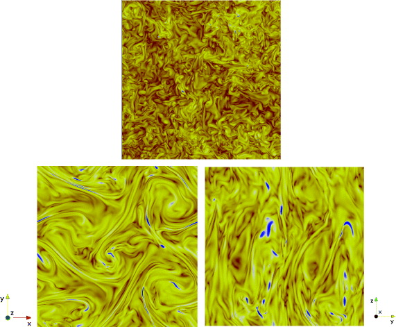
Figure 1. Typical instantaneous enstrophy densities in two-dimensional slices of the three-dimensional flows. Increasing values from red to blue. Top: isotropic turbulence (run I). Bottom: rotating turbulence (run III); left: 'horizontal' plane (perpendicular to  ); right: 'vertical' plane. The rotation vector
  is in the
z-direction.
is in the
z-direction.
Download figure:
Standard imageTable 1. Physical and numerical parameters of the runs. Reynolds number based on the Taylor microscale λ: Rλ = urmsλ/ν; large-scale Rossby number:  ; small-scale Rossby number:
  ; Zeman scale:
  . L is the integral length scale, η the Kolmogorov scale, ε is the energy dissipation rate, ν the kinematic viscosity, and urms and ωrms, respectively, denote the rms of velocity and vorticity fluctuations.
| Run | Rλ | kmaxη | Ro(L) | Ro(ω) | L/ℓZ | L/η |
|---|---|---|---|---|---|---|
| I | 190 | 1.3 | ∞ | ∞ | 0 | 165 |
| II | 270 | 1.7 | 0.12 | 1.15 | 50 | 145 |
| III | 430 | 1.9 | 0.07 | 0.55 | 140 | 125 |
The results presented in the following were obtained with runs of 5123 collocation points. The Courant number, computed as the ratio of the maximal instantaneous velocity fluctuations to δx/δt, where δt and δx are the timestep and space increment, was always <0.15. The physical and numerical parameters of these runs are gathered in table 1. Other simulations with lower resolutions (2563 and 1283) have been carried out to make sure that the observed behavior was robust.
For each of the runs I–III and each value of r0, 106 tetrads of tracer particles were considered. These tetrads were isotropic (gab = (r20/3)δab), so as to consider only one length scale. The values of r0 covered the whole inertial domain, ranging from η to L. The perceived velocity gradient tensor M was calculated through equations (1)–(3) and (5)–(8).
4. Results
4.1. Scaling laws of the low-order moments of M
The most natural statistics one can measure are the low-order moments of the M tensor. In homogeneous and isotropic turbulence, these moments are expected to satisfy approximately the Kolmogorov K41 scaling: the nth moments of M should therefore scale as (ε/r20)n/3. The ratios between different moments of the same order also give some information about the local structure of the flow. In particular, for a Gaussian ensemble of traceless matrices M,

and

In isotropic turbulence and for r0 ≳ L, the second- and fourth-order moments of M(r0) are expected to satisfy these inequalities since the velocities of the four particles are roughly uncorrelated. In statistically homogeneous turbulence, the second-order moments of the usual velocity gradient tensor mab (r0 → 0 in our case) are known to obey the exact relation 〈Ω2〉 = 2〈Tr(S2)〉. It has also been shown by DNS that the ordering (24) also holds for the m tensor in homogeneous and isotropic turbulence [38].
Figure 2 shows the second- and fourth-order moments of the M tensor measured for different Rossby numbers. As expected in homogeneous turbulence, for any Ro, the mean enstrophy 〈Ω2〉 is twice as large as the mean strain variance 〈Tr(S2)〉 for the smallest values of r0 (dissipative regime). In the isotropic case, all the moments satisfactorily satisfy the K41 prediction for scales η < r0 < L. In this type of flow, the orderings (23) and (24) are satisfied for any tetrad of size r0. Interestingly, it is found that these inequalities are also valid at any scale in rotating turbulence.
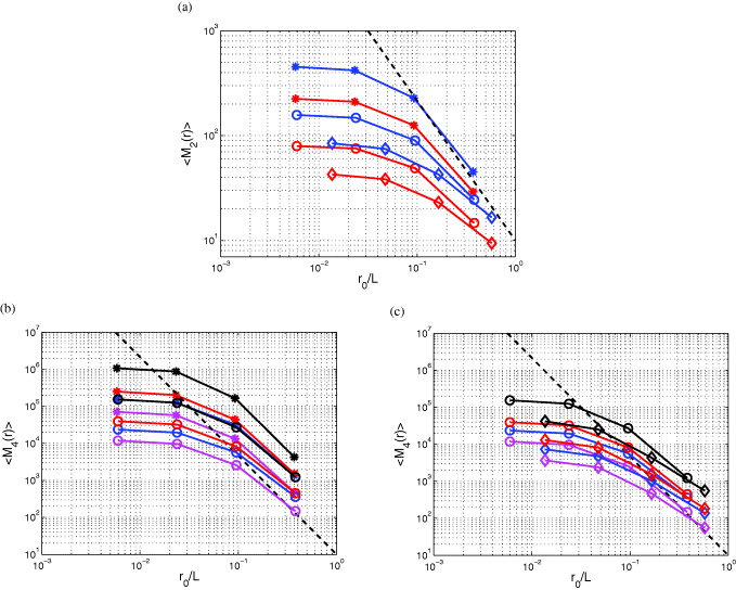
Figure 2. Scaling laws of the second- and fourth-order moments of the M tensor: *, isotropic turbulence; ○, Ro(L) = 0.12; ◊, Ro(L) = 0.07. (a) Second-order moments; blue, 〈Ω2〉; red, 〈Tr(S2)〉; dashed line, K41 prediction ∼r−4/30. (b) and (c) Fourth-order moments; black, 〈(Ω2)2〉; blue, 〈(Tr(S2)2〉; red, 〈 Tr(S2)Ω2〉; magenta, 〈ΩSSΩ〉; dashed line, K41 prediction ∼r−8/30.
Download figure:
Standard imageFigure 3 presents the third-order moments of the tensor M. Unlike the even-order moments, the third-order ones can indicate a change of sign of the velocity gradient, and thus provide information on the asymmetry of the structures in the flow. A term such as 〈ΩSΩ〉 is involved as production in both the strain equation (16) and the vorticity equation (20), and is compared to 〈 − Tr(S3)〉 in figure 3(a). For both the rotating cases and the isotropic one, |〈 − Tr(S3)〉| > |〈ΩSΩ〉|, with a K41 scaling recovered in the isotropic case (not shown here), and a positive production 〈ΩSΩ〉 > 0. The production term 〈 − Tr(S3)〉 in the strain variance equation also remains positive at all Rossby numbers, but 〈ΩSΩ〉 is much reduced, with a value within the statistical sampling jitter for the most rapidly rotating case. This term is therefore compared in figure 3(b) to the other vorticity production term in the enstrophy equation,  , due to background rotation. The latter term is still smaller than 〈ΩSΩ〉, and we note that some sign reversal can occur, particularly clear in the case of larger Rossby number. This may be due to a change in the dynamics at large scales, where rotation is comparatively more active, with respect to the smaller scales in which the perceived velocity gradients become less influenced by rotation progressively when approaching the dissipative scales, with a return to isotropy. The last panel (c) of figure 3 shows, in addition, the third production term in the strain variance equation,
  . For all cases, this term is smaller than the other two, according to
  .
.
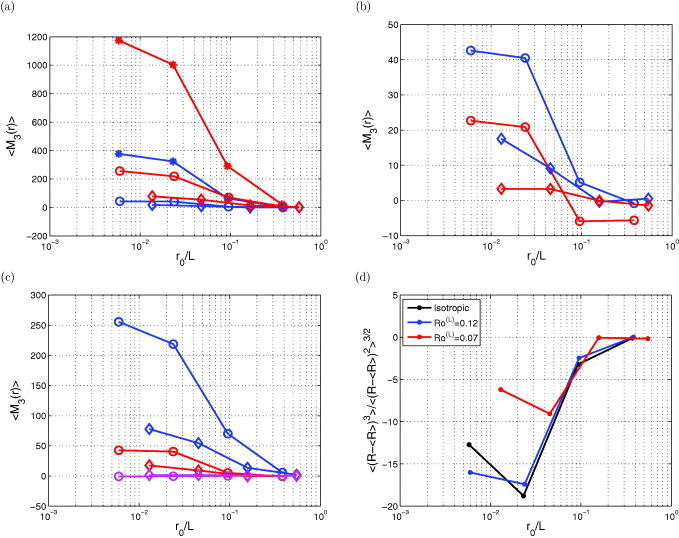
Figure 3. Scaling laws of the third-order moments of the M tensor: *, isotropic turbulence; ○, Ro(L) = 0.12; ◊, Ro(L) = 0.07. (a) Blue, 〈ΩSΩ〉; red, 〈 − Tr(S3)〉. (b) Blue, 〈ΩSΩ〉; red,  . (c) Blue, 〈 − Tr(S3)〉; red, 〈ΩSΩ〉; magenta,
  . (d) Skewness of R for the isotropic and rotating cases.
Download figure:
Standard imageTo sum up the salient scaling properties, the K41 laws are reasonably recovered for the second- and fourth-order moments of the M tensor. The third-order moments are those that can be most affected by rotation, through two possible contributions:  directly proportional to the rotation rate, and the nonlinear modification of the dynamics of energy transfer that affect the other third-order moments.
4.2. Joint probability density functions of Q and R
Figure 4 shows the joint probability density function (PDF) of the R and Q invariants for different values of r0 ranging from L/3 to η, in isotropic turbulence. In agreement with the literature [16, 19], this PDF is almost symmetric with respect to the R = 0 axis at large scale, and gets more and more skewed as the scale decreases. For r0 ≈ η, the well-known 'tear-drop shape', with an excess of probability along the R > 0 side of the zero-discriminant line (Vieillefosse tail), is recovered. The same quantities are plotted in figure 5 for the rotating case at Ro(L) = 0.12. Interestingly, the PDFs at small scale are qualitatively very similar to those obtained in isotropic turbulence (see, e.g., figures 4(d) and 5(d)). This is not the case at large scale (figures 4(a) and 5(a)), where the PDF measured in rotating turbulence is much more symmetric with respect to the R = 0 axis, i.e. closer to a Gaussian distribution [16]. In particular, we found that, in rotating turbulence, the joint PDF of R and Q at scales larger than ℓZ, the Zeman scale, are much more symmetric than their counterparts in isotropic turbulence, whereas these quantities at scales smaller than ℓZ are qualitatively very similar to the isotropic ones. This observation is confirmed by figure 6 at Ro(L) = 0.07, in which all the scales are >ℓZ and thus are affected significantly by rotation.

Figure 4. Joint PDF of the normalized R = −Tr(M3)/3 and Q = −Tr(M2)/2 invariants: R* = R/〈(Tr(S2))3/2〉, Q* = Q/〈Tr(S2)〉, in isotropic turbulence. (a) r0 ≈ L/3; (b) r0 ≈ L/11; (c) r0 ≈ L/43 ≈ 4η; (d) r0 ≈ L/170 ≈ η. The isoprobability contours represent the probabilities 10−n, where n is an integer (see colorbars). The dashed line is the zero-discriminant line: 27R2 + 4Q3 = 0.
Download figure:
Standard image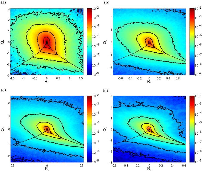
Figure 5. Joint PDF of the normalized invariants R* and Q*, for Ro(L) = 0.12. (a) r0 ≈ L/3 ≈ 18ℓZ; (b) r0 ≈ L/11 ≈ 5ℓZ; (c) r0 ≈ L/44 ≈ 3η ≈ ℓZ; (d) r0 ≈ L/180 ≈ 0.8η ≈ 0.3ℓZ. The same conventions as in figure 4.
Download figure:
Standard image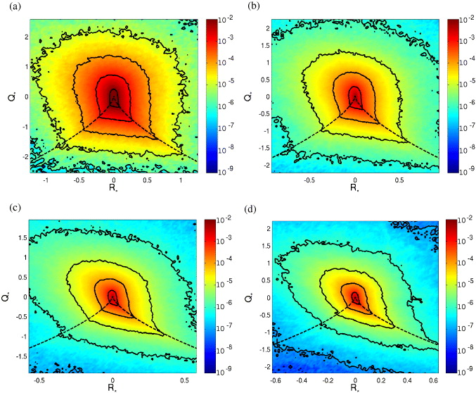
Figure 6. Joint PDF of the normalized invariants R* and Q*, for Ro(L) = 0.07. (a) r0 ≈ L/2; (b) r0 ≈ L/6; (c) r0 ≈ L/21 ≈ 6η; (d) r0 ≈ L/73 ≈ 1.5η. All these scales are larger than ℓZ. The same conventions as in figure 4.
Download figure:
Standard imageRotation has already been identified in the model proposed by Li [15] as responsible for the modification of the PDF of the passive scalar gradient in turbulence, by strongly reducing strong events and thus restoring a PDF much closer to Gaussian distribution than in isotropic turbulence, for sufficiently large rotation rates (Ro(ω) = 0.2 in [15]). Our results presented in figure 3(d) show the skewness of R, Sk(R) = 〈(R − 〈R〉)3〉/〈(R − 〈R〉)2〉3/2, as a function of scale. Sk(R) is reduced in the inertial range when rotation is sufficiently large at Ro(ω) = 0.55 (also Ro(L) = 0.07), and almost no change is observed between the isotropic and the rotating case at Ro(ω) = 1.15. (Note that accurate statistical convergence is difficult to reach for these statistics.) From a phenomenological point of view, inertial waves may be invoked to explain the Gaussianization of the PDF distribution. For the strongly rotating case of run III, the local Rossby number at large scales is much smaller than unity, indicating the dominance of rotation effects over turbulent transport or, in other words, of the linear effect of rotation over nonlinear advection. Therefore, the velocity field is strongly influenced by the propagation of inertial waves with only weak nonlinear interactions. To illustrate this, one may consider the linearized equations (21) applied to an initial Gaussian field. In that case, no departure from Gaussianity is expected from the propagation of waves. A small departure may be observed for weakly interacting waves, whereas the full nonlinear regime is required to produce a non-Gaussian field with non-zero third-order moments. When rotation is weaker, the Rossby number at large scales is larger, indicating less effective linear wave propagation against nonlinear transport.
4.3. Densities of second-order moments of M in the (R, Q) plane
More refined information about the local structure of turbulence can be gained by plotting the densities of dynamical quantities in the (R, Q) plane, defined as the conditional PDF on Q and R multiplied by the joint PDF of these invariants. This permits us to link the intensity of the corresponding statistical quantity to the topological structure of the flow, depending on the location of its concentration with respect to the separatrix and to the R = 0 axis in the (R, Q)-plane.
We investigate first the second-order moments of the M tensor. Figures 7 and 8, respectively, show the densities of strain variance, Tr(S2), and of enstrophy, Ω2, in the (R, Q) plane, for several values of the tetrad size r0 and of the Rossby number. These two quantities are always essentially concentrated around the origin. As expected and already observed in isotropic turbulence, the enstrophy density mostly extends in the region D > 0, corresponding to elliptic flows. Rotation does not seem to strongly influence these observables. The strain variance density is simply more elongated along the R > 0 side of the separatrix D = 0 for small tetrad sizes and low rotation rate, in accordance with the joint PDF of Q and R.
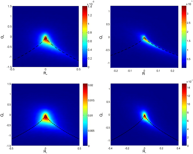
Figure 7. Density of Tr(S2) (strain variance), normalized by its average, in the (R*, Q*) plane. Top: isotropic turbulence; bottom: Ro(L) = 0.07. Left: r0 ≈ L/3; right: r0 ≈ η.
Download figure:
Standard image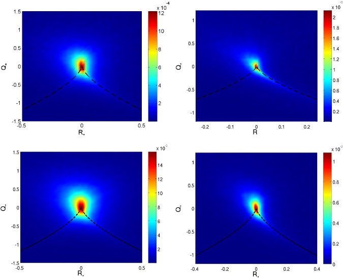
Figure 8. Density of enstrophy, Ω2, normalized by its average, in the (R*, Q*) plane. Top: isotropic turbulence; bottom: Ro(L) = 0.07. Left: r0 ≈ L/3; right: r0 ≈ η.
Download figure:
Standard image4.4. Densities of third-order moments of M in the (R, Q)-plane
We expect the effect of rotation to be more significant on statistics related to third-order moments of M, since previous studies of the dynamics of rotating turbulence in spectral space [28] have indicated that third-order velocity moments are nonlinearly affected by rotation, which does not alter the spectral energy distribution, a second-order velocity moment.
We consider the strain skewness −Tr(S3) appearing in the strain variance equation, and plot its conditional PDF in figure 9. As expected, the isotropic case shows a large- and a small-scale positive concentration which lie along the R > 0 part of the D = 0 separatrix, i.e. along sheets. At a large scale, regions of negative concentration are visible along the R < 0 part of the separatrix (filaments), but the net balance 〈 − Tr(S3)〉 is positive. In isotropic turbulence, this quantity is a good approximation of the energy transfer −Tr(M2Mt) [16]. Positive (resp. negative) concentrations of these quantities therefore correspond to regions of local direct (resp. inverse) energy cascade. In the strongly rotating case at Ro(L) = 0.07, −Tr(S3) is only very slightly more concentrated toward R = 0 (this is related to the joint PDF of the R and Q invariants, qualitatively different in both flows, see figures 4 and 6), but it is clear that the strain skewness is almost not influenced by rotation throughout all scales.
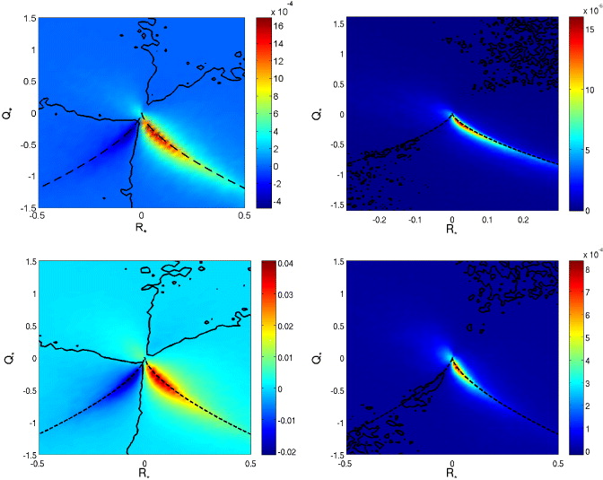
Figure 9. Density of −Tr(S3) (strain skewness), normalized by the absolute value of its average, in the (R*, Q*) plane. Top: isotropic turbulence; bottom: Ro(L) = 0.07. Left: r0 ≈ L/3; right: r0 ≈ η.
Download figure:
Standard imageThe distribution of conditional PDF of the term ΩSΩ (enstrophy production in isotropic turbulence) is plotted in figure 10, for the isotropic and strongly rotating cases. In the left panels, corresponding to the large scales, ΩSΩ is positive in vorticity filaments, and negative in vortex sheets. The background value is recovered in the hyperbolic zone, below the separatrix in the (R, Q) plane. In the isotropic case, enstrophy is therefore essentially produced in vorticity filaments, and destroyed in vortex sheets, as already observed experimentally [39]. At smaller scales r0 ≈ 4η, rotation seems to modify the ΩSΩ distribution very weakly by spreading its positive and negative peaks, although this trend is blurred by the statistical noise.

Figure 10. Density of ΩSΩ (enstrophy production in the isotropic case), normalized by the absolute value of its average, in the (R*, Q*) plane. Top: isotropic turbulence; bottom: Ro(L) = 0.07. Left: r0 ≈ L/3; right: r0 ≈ 4η.
Download figure:
Standard imageThe density of the conditional PDF of  (figure 11) shows that it is positive in filaments of vorticity, and negative in vortex sheets or in strain sheets, and not much influenced by the rotation rate.
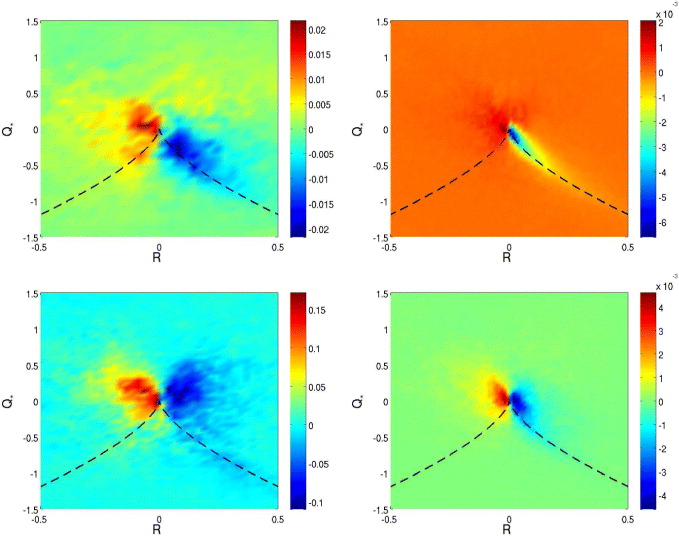
Figure 11. Density of  , normalized by the absolute value of its average, in the (R*, Q*) plane. Top: Ro(L) = 0.12; bottom: Ro(L) = 0.07. Left: r0 ≈ L/3; right: r0 ≈ 4η.
Download figure:
Standard imageFinally, the density of the conditional PDF of  is shown in figure 12: the large-scale plots exhibit a wide negative patch around the origin, which corresponds to a marked 'sink' of enstrophy. The smaller scale distribution shows that this enstrophy production term related to background rotation is negative in vorticity filaments, and positive for vortex and strain sheets. Interestingly, this behavior is completely opposite to that of the isotropic enstrophy production ΩSΩ (see figure 10). Overall, this shows that rotation might therefore be able to alter the enstrophy balance, or enstrophy cascade, between the large and the small scales.
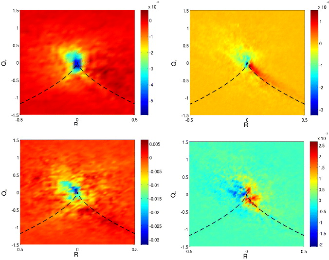
Figure 12. Density of  , normalized by the absolute value of its average, in the (R*, Q*) plane. Top: Ro(L) = 0.12; bottom: Ro(L) = 0.07. Left: r0 ≈ L/3; right: r0 ≈ 4η.
Download figure:
Standard imageWhen  is superimposed with the enstrophy production term ΩSΩ, one obtains the total enstrophy production (see equation (20)), plotted in figure 13. The figure shows that at a small Rossby number, or at a large Rossby number and a large scale (figures 13(a), (c) and (d))—i.e. when r0 > ℓZ— the distribution of total enstrophy production is very similar to that of
  , which is therefore the dominant term. Otherwise, at r0 < ℓZ (figure 13(b)), ΩSΩ is dominant and the distribution of the total production is closer to the enstrophy production distribution observed in isotropic turbulence, positive in vorticity filaments and destructive (negative) in vortex sheets.

Figure 13. Density of  (total enstrophy production in rotating turbulence), normalized by the absolute value of its average, in the (R*, Q*) plane. Top: Ro(L) = 0.12; bottom: Ro(L) = 0.07. Left: r0 ≈ L/3; right: r0 ≈ 4η.
Download figure:
Standard imageTo complete the analysis of the dynamics, we plot in figure 14 the total production of strain variance (see equation (16)). As expected from figure 3, the contribution of −Tr(S3) is always larger than the others, so that the distribution of this total production of strain remains similar to that of isotropic turbulence, since the distribution of this quantity is very weakly dependent on the Rossby number (see figure 9): the positive contributions are located in vortex sheets and in strain sheets, and some destruction due to negative contributions is present in filaments, although the overall net balance is positive; it is thus a net production term.
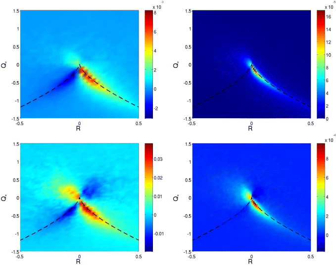
Figure 14. Density of  (total production of strain variance in rotating turbulence), normalized by the absolute value of its average, in the (R*, Q*) plane. Top: Ro(L) = 0.12; bottom: Ro(L) = 0.07. Left: r0 ≈ L/3; right: r0 ≈ 4η.
Download figure:
Standard image5. Conclusion
The anisotropy of rotating homogeneous turbulence stems from a rather intricate effect of rotation, which was shown in previous works to act on energy transfers at the level of third-order velocity moments, and not directly on the energy distribution, due to the fact that the Coriolis force does not produce work. Therefore, the statistical analysis of rotating turbulence is quite complex, since it has to deal with higher-order statistics than energy spectra, and scale-dependent effects of rotation. The latter have to be parameterized by the Zeman scale, in addition to the more global Rossby number, either based on the large scales or based on the Taylor microscale. The analysis we have proposed, based on the statistics of the perceived velocity gradient tensor M, interpolated from the locations and velocities of an isotropic tetrad of fluid particles of dimension r0, addresses nicely all these constraints: (a) it allows for a multi-scale analysis, by choosing the coarse-graining scale r0 for the velocity gradient, which we have mostly set slightly smaller than, or close to, the integral length scale L, or slightly larger than, or close to, the dissipative Kolmogorov scale η; (b) it permits to compute the production terms in the enstrophy equation, or in the strain variance equation, and to evaluate their relative strengths. In addition, the analysis of the invariants of the perceived velocity gradient tensor permits us to link the peaks of the production terms with the structural features of the flow, since the (R, Q) plane distribution of the PDF of these dynamical quantities can be examined in specific topological zones: vortex sheets, strain sheets, vortex filaments, thanks to the D = 0 separatrix between elliptic and hyperbolic regions and to the R = 0 axis separating one-dimensional (filaments) from two-dimensional (sheets) structures.
We have performed a statistical analysis of the data from DNS of forced rotating homogeneous turbulence. The forcing is based on a subset of the Euler equations, coupled with our Navier–Stokes pseudo-spectral algorithm with Fourier polynomials. The forcing is therefore 'natural' in that it does not introduce any external length or timescale which would be imposed on the flow. Thus, the obtained rotating turbulence reaches rather high Reynolds numbers, up to Rλ = 430, and we have chosen a moderately small Rossby number case and a rapidly rotating case at smaller Rossby number, in addition to the reference isotropic case. The rotating flow structure we present is clearly strongly anisotropic, with features in horizontal planes strongly resembling two-dimensional turbulence, but with strong vertical gradients when examining vertical plane cuts of the velocity field. Thanks to the achieved Reynolds numbers, we were able to recover scaling laws for the second- and fourth-order moments of M consistent with the prediction by Kolmogorov [40], uniformly for the rotating and non-rotating cases. Unlike its even-order moments, the third-order moment of M is shown to be influenced by rotation and may even become negative depending on the non-dimensional parameters and the scale.
The joint probability distribution function of the invariants R and Q of M recover the elongation along the 'Vieillefosse' tail for the small scales already observed in isotropic turbulence, leading to the 'tear-drop-shaped' distribution. In rotating flows, no significant modification of this distribution is observed at scales smaller than the Zeman one. But at scales larger than ℓZ (i.e. at all scales at small Rossby number Ro(L) = 0.07, and at the largest scales only at moderate rotation rate, where Ro(L) = 0.12), the distribution is more symmetric with respect to the R = 0 axis, a signature of a Gaussian distribution, than the one measured in isotropic turbulence. A possible explanation is the increased presence and effect of inertial waves, rendering the dynamics closer to that of wave turbulence, in which the closeness to Gaussianity is a feature of the velocity field, with less important nonlinearity in the energy transfers.
In order to investigate further the sources of these dynamical modifications due to rotation, we have presented PDFs of statistical terms appearing in the strain variance and enstrophy equations, conditioned by the R, Q distribution. As expected, the influence of rotation on the strain variance itself and the enstrophy (second-order moments) is rather weak at both the presented scales L/3 and η (and at all the computed scales not plotted here). Regarding the production terms (third-order moments), not all are noticeably affected by rotation, such as the strain skewness term −Tr(S3). The distribution in the (R, Q) plane of enstrophy production ΩSΩ is moderately changed by rotation at all scales, and retains its isotropic shape, as does the total production in the strain variance equation. When combined with the production due to background rotation  to yield the total enstrophy production in rotating turbulence
  , it shows the importance of the relative amplitude of the tetrad scale r0 with respect to the Zeman scale ℓZ. The latter therefore appears as a fixture in rotating homogeneous turbulence, although it needs to be discussed along with dynamical terms—e.g. production terms in the enstrophy equation or third-order velocity structure function in the Kármán–Howarth equation or spectral energy transfer in the Lin equation—in order to complete the analysis of the full Eulerian properties of rotating homogeneous turbulence.
It is also important to note that the distribution of the total production of strain variance (figure 14) is a rather robust feature, since, in rotating turbulence, it remains very close at all scales to that of isotropic turbulence.
In this work, we have focused on fixed tetrads of fluid particles, but the same approach will be used in a forthcoming study by following the trajectory of each fluid particle of the initial tetrad and thus gaining access to Lagrangian statistics of the ρ and M tensors.
Acknowledgments
We are grateful to A Pumir and C Cambon for stimulating discussions. The study was completed using the resources of GENCI-IDRIS (grant numbers 2011022206 and 2012022206). This work has been supported by the Agence Nationale pour la Recherche under contract numbers 08-BLAN-0076 'ANISO' and 07-BLAN-0155 'DSPET'.