

Abstract
Origami provides a flexible platform for constructing three-dimensional multi-stable mechanical metamaterials and structures. While possessing many interesting features originating from folding, the development of multi-stable origami structures is faced with tremendous demands for acquiring tunability and adaptability. Through an integration of origami folding with magnets, this research proposes a novel approach to synthesize and harness multi-stable magneto-origami structures. Based on the stacked Miura-ori and the Kresling-ori structures, we reveal that the embedded magnets could effectively tune the structure's potential energy landscapes, which includes not only altering the position and the depth of the potential wells but essentially eliminating the intrinsic potential wells or generating new potential wells. Such magnet-induced evolutions of potential energy landscapes would accordingly change the origami structure's stability profiles and the constitutive force–displacement relations. Based on proof-of-concept prototypes with permeant magnets, the theoretically predicted effects of magnets are verified. The exploration is also extended to the dynamics realm. Numerical studies suggest that the incorporated magnets not only could translate the critical frequencies for achieving certain dynamical behaviors but also fundamentally adjust the frequency-amplitude relationship. Overall, this study shows that the proposed approach would provide a novel means to control the stability profile as well as the mechanics and dynamic characteristics of origami structures, and thus, inspire new innovations in designing adaptive mechanical metamaterials and structures.
Export citation and abstract BibTeX RIS
1. Introduction
Multi-stability, characterized by coexisting potential energy minima for a given set of parameters, has led to a revolution in developing artificial structures and materials with multifarious adaptive functionalities. Kinematically, multi-stable materials and structures could remain at different stable configurations without external aids, letting them immediately attractive in various shape morphing applications [1–4]. They could also feature different mechanical properties at different stable equilibria that allow us to online tune the performance by strategically switching the states, including auxetic regulation [5–7], stiffness and damping adaptability [8–12]. Under external excitations, multi-stability will trigger rich dynamic behaviors that could be exploited for function improvements, including fast actuation that makes use of the snap-through jumps [13, 14], energy harvesting that takes advantages of the large-amplitude inter-well oscillations [1, 15, 16], vibration control benefiting from the low-amplitude intra-well oscillations or excitation-induced stability [16–18], robust sensing as a result of the bifurcation phenomena [16, 19, 20], and non-reciprocal wave propagation profiting from the unique asymmetric bi-stability [21–24]. Therefore, incorporating multi-stability has become a promising and effective way of developing high-performance structures and functional materials with adaptivity.
In spite of the intriguing attributes and the enormous potentials of multi-stable structures and materials, the constituent units for achieving multi-stability are very similar, concentrating on the curved or pre-stressed bi-stable springs, beams, arcs, shells, and their close relatives. Such architectures show simplicity in designing, modeling, mechanical analysis, and fabrication because their bi-stability is mainly evident in one direction. Through topology analyses, these units can be further tessellated into two-dimensional (2D) or three-dimensional (3D) lattice configurations [2, 25, 26]. However, they are also facing inevitable limitations that their underlying mechanisms of bi-stability remain essentially the same, i.e. elastic buckling instability [25], and these component units are scarcely capable of being assembled into truly 3D systems with diverse geometry forms. These deficiencies may weaken the overall potentials of multi-stable systems, which, therefore, raise desperate demands for new constituent units for constructing complex 3D configurations as well as novel principles for achieving multi-stability.
Recently, origami, the art of paper folding, has been identified as a powerful platform for constructing and transforming 3D shapes as well as achieving multi-stability. Unlike the conventional strategies that are monotonous in terms of the underlying mechanisms and representations, origami folding provides fundamentally different principles and rich design resources toward 3D multi-stable structures. For example, the stacked Miura-ori (SMO) structure, assembled by two Miura-ori cells with kinematic constraints, is essentially a 3D structure featuring a double-well potential landscape by elaborately prescribing the crease patterns and precisely assigning the crease stiffness. Its fundamental bi-stable mechanism has been recognized as the non-unique correspondence between the folding angles of the two constituent Miura-ori cells [27]. Connecting multiple SMO units in series or in parallel, more potential energy minima (i.e. multi-stability) and even mechanical diode effect [28–30] can be obtained. In generic degree-4 vertex origami cells, the nonlinear relationship between folding angles would also induce complex potential landscapes with as many as five minima [31]. In these examples, rigid foldability is ensured that the facets keep undeformed during folding but just rotate around the hinge-like creases. Breaking the rigid-foldability pre-condition, multi-stability can also be acquired in non-rigid-foldable origami structures on account of the elastic facet deformations and the nonlinear geometries, such as the square-twist pattern [32], the Kresling origami structure [33], and the origami ball [34]. Therefore, by offering both sophisticated 3D geometries and rich mechanisms of multi-stability, the origami solution could potentially overcome the intrinsic limitations of the conventional 1D/2D multi-stable structures, bring about novel characteristics and functionalities, and find broad application prospects.
Note that the multi-stability is always an inherent property if the structure design and the component materials are pre-determined. In other words, for a given multi-stable structure, its underlying potential energy landscape cannot be quantitatively modified or qualitatively changed. However, a controllable multi-stability profile without re-designing and re-fabricating the prototype is desirable in applications. For example, if the depths of the potential wells are quantitatively changeable, the critical force for switching the structure between adjacent stable configurations would become tunable for specific needs. If the number and positions of potential wells are qualitatively adjustable, adaptive structures and materials with tailorable stable configurations can be developed for customized shape morphing. Controlling multi-stability also has dynamics significance. Taking energy harvesting as an example, if the environmental vibrations are weakened, large-amplitude inter-well responses can still be attained in a bi-stable system by reducing the potential well depths [35]; otherwise, if with intense environmental vibrations, energy harvesting performance can be further improved via upgrading the system from bi-stable to multi-stable [36]. For origami, the above arguments also hold; a given origami structure with pre-specified crease pattern and constituent materials can only exhibit a constant stability profile, and evolution to a controllable one will be desirable and significant.
To achieve such controllability, additional components are needed to be incorporated into the origami structure. For example, previous research reveals that the multi-stability characteristics can be effectively tuned by fluidic pressure. Upon pressurization, a SMO structure can switch its energy landscape between mono-stable and bi-stable; by stacking two pressurized cells, more than two stable states can be generated [29]. While showing promising results, the pressure solution requires a hermetic chamber inside the origami structure as well as cumbersome pressure regulating devices, which severely limits its application. Inspired by the facts that magnets are widely exploited in classical mechanical devices to achieve and to harness multi-stability, this research proposes employing magnets to control the stability profiles of origami structures. Note that coupling of origami and magnets has already been explored in previous research in terms of magnetic actuation and self-folding [37–40]. However, the effects of magnets on origami structures' stability profiles and mechanical properties have not been studied.
In this research, by integrating magnets with origami structures at prescribed geometric entities, magneto-origami structures with diverse magnet arrangements and pole layouts are demonstrated. The stability profile of the coupled structure is determined by both the elastic and the magnetic potential energies. Here, the overall potential landscape, and hence, the stability profile, can be quantitatively or even qualitatively tailored by tuning the magnetic field strength or the magnetic polarization. Observed phenomena include the quantitative changes of potential well depths, migrations of potential well positions, and evolutions among single-well, double-well, and triple-well landscapes (corresponding to mono-stable, bi-stable, and tri-stable profiles, respectively). Such changes of stability profile would, in turn, affect the constitutive force–displacement relation and induce drastically different dynamic responses, thereby illustrating the significance of the magnet approach in applications.
Foreseeable advantages of the proposed approach are multiple. First, the magnets can be compactly embedded with origami structures at rich geometric entities (e.g. on vertices or facet centers, etc), offering great design flexibility. Second, the magnetic effect is largely reliable and robust, making this approach feasible in diverse working environments and suitable for various applications. Third, tuning the magnetic strength and magnetic polarization can be easily achieved by adjusting the currents if electromagnets are employed; as a proof-of-concept study, this research uses permanent magnets in theoretical and experimental analyses to uncover the underlying mechanisms of multi-stability and to reveal the effects of magnets on statics and dynamics.
In the following sections, the rich design of origami magnetic-elastic integration is first introduced, exemplified by the SMO structure and the Kresling-ori structure (section 2). Theoretical results are then reported to demonstrate how magnets could quantitatively and qualitatively control the stability profile and affect the static characteristics (section 3), which are experimentally verified based on proof-of-concept prototypes with permanent magnets (section 4). Following that, numerical studies are carried out to illustrate the magnet-induced evolutions of the magneto-origami structures' dynamic characteristics (section 5). Finally, summary and conclusions are presented (section 6).
2. Origami magnetic-elastic integration
Origami structures could offer abundant vertices, creases, and facets for embedding magnets. Note that a generic guideline for arranging magnets in origami structures does not exist, and with different embedding positions and manners, the magnetic-elastic coupling would present significant differences that cannot be simply quantified by a parameter. In this section, we use the SMO structure and the Kresling-ori structure to exemplify the rich design possibilities of magnetic-elastic integration. For ease of use, the geometries of the Miura-ori and the Kresling-ori are provided without detailed derivations.
2.1. Magnetic-elastic coupled Miura-ori structures
Miura-ori pattern is a kind of degree-4 vertex crease pattern with a pair of collinear creases and reflectional symmetry. Two Miura-ori cells with kinematic compatibility can be assembled into a SMO structure [41, 42]. The bottom and the top Miura-ori cells are characterized by crease lengths  and
and  and a sector angle
  where
where  takes 'A' or 'B', denoting the bottom cell A and the top cell B, respectively (figure 1(a)). They have to satisfy the following kinematic compatibility conditions

Folding of the SMO structure is a one degree-of-freedom (DoF) mechanism that can be described by the folding angles  or
or  they are not independent to each other but satisfy

The outer dimensions of the SMO structure, i.e. the length  the width
  and the height
  can be expressed in terms of
  (here and in what follows, the subscript 'M' denotes the Miura-ori)
Folding of the structure can also be characterized by the dihedral angles between facets  and the dihedral angles at the connecting creases
  where
where  and
and  (figure 1(a)). They can also be expressed as functions of
Based on whether the bottom cell A nests into or bulges out from the top cell B, the SMO structure could exhibit two qualitatively different configurations. For clarity, the configurations with  and
and  are denoted as nested-in and bulged-out, respectively (figure 1(a)).

Figure 1. Geometries and designs of the magnetic-elastic coupled Miura-ori structures. (a) Geometries of the stacked Miura-ori (SMO) structure. The mountain and valley folds in the crease pattern are denoted by dashed and dotted–dashed lines, respectively; the vertices in the stacked structure are denoted by numbers from '1' to '12'; the folding angles  the dihedral angles
 and the outer dimensions (

 ) are also indicated. (b) Three different designs (I, II, and III) for embedding magnets, where the magnetic poles are not denoted. (c) Two different pole layouts of Design I. (d) Five different pole layouts of Design II. (e) Four representative pole layouts of Design III, where the colors denote the poles facing inside the stacked structure.
Download figure:
Standard image High-resolution imageAn SMO structure possesses 12 vertices, 20 creases, and 8 facets that can be employed for magnet integration. Figure 1(b) displays three different designs for embedding magnets. In Design I, two magnets are placed at the top vertex '2' and the bottom vertex '11'; in Design II, four magnets are positioned at four coplanar vertices ('4', '6', '7', '9'); in Design III, eight magnets are embedded at the facet centers. In addition to changing the magnet arrangement, the design can be further enriched by adjusting the magnetic polarization. In Design I, the two magnets can be set with their like poles or opposite poles facing each other, giving rise to the repulsive-magnet and the attractive-magnet layouts, respectively (figure 1(c)). In Design II, the four coplanar magnets can make up 16 different pole layouts, which can be deducted into 5 by considering the symmetry among the four magnets and the identity among certain pole-pole relationships (figure 1(d)). In Design III, the 8 magnets could constitute variegated 3D pole layouts; for demonstration purpose, a few examples are given in figure 1(e).
During folding ( varies between
  and
and  ), the outer dimensions of the SMO structure would experience significant changes [41, 42], which would, therefore, alter the relative distances among the magnets and change the system's stability profile. This will be detailed in section 3.
2.2. Magnetic-elastic coupled Kresling-ori structures
The crease pattern of a Kresling-ori [33] is made up of a row of  identical parallelogram panels, each parallelogram panel is defined by three length parameters:
  and
and  are the side lengths,
  is the length of the long diagonal (here and in what follows, the subscript 'K' denotes the Kresling-ori) (figure 2(a)). Construction of the structure from the flat crease pattern is achieved by folding and rolling it into a polygonal prism such that points 'A' and 'B' overlap with 'A*' and 'B*'. Geometries of the folded structure can be described by the circumradius of the basal polygon
  the height
  and the relative rotation angle
  of the top polygon with respect to the frame fixed to the bottom polygon (figure 2(b)). Variation in the polygon circumradius
  would scale the size of the origami; the height
  or the rotation angle
  are used to characterize the structure configuration.

Figure 2. Geometries and designs of the magnetic-elastic coupled Kresling-ori structures. (a) The crease pattern of a Kresling-ori (
 ), where the mountain and valley folds are denoted as dashed and dotted–dashed lines. (b) A Kresling-ori structure based on the pattern shown in (a) (left) and the top-down view of the structure (right). Rotation of the top octagon with respect to the frame fixed to the bottom octagon is described by the angle
  which is measured from the
  -axis to the vector
  The origin of the frame locates at the center of the bottom octagon, and the x-axis is chosen to intersect vertex 'A' of the bottom octagon. (c) Folding of the Kresling-ori structure between the 'open' and the 'closed' configurations, where evolutions of the height
  and the rotation angle
  are shown. (d) The vectors in a unit panel
  which are used for determining the folding motion. (e) Introducing virtual folds
  and
and  to account for the panel bending. For readability of the figure, only the virtual folds in the unit panel
  are plotted. (f) A design for embedding magnets, where the colors denote the poles facing inside the Kresling-ori structure; two magnetic pole layouts are given: the repulsive-magnet layout (left) and the attractive-magnet layout (right).
Download figure:
Standard image High-resolution imageTo quantify the aspect ratio of the structure and the degree of transformation during folding, an angle ratio  is defined, which is the ratio of the angle
  to half the internal angle of the basal polygon
  The value of
  is bounded by
  [33], where the lower bound indicates a limiting case that the structure height
  constructed from two offset polygon bases connected by triangular panels, and the upper bound indicates a limiting case that the parallelogram panels become rectangular panels such that
  With a smaller value of
  the structure height
  and the rotation angle
  vary less during folding.
  indicates a change in chirality, i.e. anticlockwise rotation of the top polygon will result in an expansion of the structure. Negative and positive chirality are mathematically identical; hence, situations with
  are not considered here. With parameters
 and
and  the remaining lengths and angles (
 and
and  ) can be determined from the crease pattern (figure 2(a)), the folded structure, and the basal polygon (figure 2(b)):
Note that each vertex in the Kresling-ori crease pattern has one DoF. Hence, for  overlapping of the vertices 'A', 'B', and 'A*', 'B*' could generate an 'open' or a 'closed' polygonal prism via rigid folding. However, if these overlapped vertices are fixed together (e.g. by gluing), the relative position of each vertex with respect to its neighbors will be fully defined, and the generated structure will be kinematically rigid at either the 'open' or the 'closed' configuration. That is, if the triangular panels are truly rigid, the expanded polygonal prism cannot be contracted, and vice versa. Only if the panels or the creases are deformable, the structure is possible to exhibit snapping transformations between the 'open' and the 'closed' configurations (figure 2(c)). Applying a force on the top of the structure and allowing free rotation, the structure will twist and contract; inversely, applying a pull force on the top, the structure will twist and expand. Note that such folding of the Kresling-ori structure is no longer rigid.
To determine the structure configuration, i.e. the height  and the rotation angle
  the following vector loop equation and kinematic constraint equations (figure 2(d)) have to be satisfied [33]:
Constraint 1 implies that the angle between  and
and  is a constant
  Constraint 2 indicates that the fold
  is rigid so that its length remains a constant
  (in this paper,
  denotes the Euclidean length). In addition, the length of the fold
  is mathematically assumed to be variable, so that an additional DoF is introduced that allows the structure to be foldable between the open and the closed configurations. Detailed procedures for determining the folding kinematics are briefly summarized as:
- Step 1:Solve the initial rotation angle
 via the vector loop equation and Constraint 1;
 - Step 2:Solve the initial height via Constraint 2;
- Step 3:Solve the final rotation angle via Constraint 2 and with
- Step 4:Let varies between and with step i.e. solve via Constraint 2 at each
- Step 5:With and calculate the strain in the crease based on


The value of  is a direct measure of the structure's non-foldability and bi-stability; however, Pagano et al [33] has pointed out that the assumed strain
  cannot properly reflect the observed deformation of a paper Kresling-ori structure, rather, with a relief cut along the fold
  bending of the triangular panels
  and
and  can better describes the facet deformations. Thus, two virtual folds,
  and
and  are mathematically added across each kinematically rigid panel (figure 2(e)) to capture the panel bending [32, 33, 42]. In this way, the rigid triangular panels
  and
and  are divided into four rigid triangular facets:

 and
and  Note that the triangular facets
  and
and  can be considered as rotations of
  and
and  they are mathematically redundant. In what follows, only the virtual fold
  is examined.
The position of the virtual fold  i.e. the position of the virtual vertex V, can be set arbitrarily on the crease
  During folding, its spatial position can be determined based on the following constraints [33]:
Constraint 3 indicates that the lengths of sides  and
and  sum to the length of the crease
  Constraint 4 asks that the length of the virtual fold
  remain constant
  during folding, where
  is determined from the open configuration; Constraint 5 is the Cosine rule of the triangle
  that determines the out-of-plane deflection, where the length
  is obtained from the strain
 and
and  remain fixed. By solving the constraint equation (7), the position of the virtual vertex
  as well as the dihedral angles at folds
 and
and  (i.e.
(i.e. 
 and
and  ) can be determined.
The Kresling-ori structure shown in figure 2(b) possesses 8 vertices and 8 sides on the top layer, as well as 8 vertices and 8 sides on the bottom layer that can be employed for embedding magnets. Figure 2(f) shows a design example, in which 8 magnets are embedded on the top-layer vertices, and 8 magnets are embedded in the bottom-layer side centers. As the two easiest pole layouts, the top-layer and bottom-layer magnets can be set with their like poles or opposite poles facing each other, giving rise to the repulsive-magnet layout and the attractive-magnet layout (figure 2(f)). Other designs and magnetic pole layouts are also possible but are not considered in this research.
During folding, in addition to the height change, the top layer would rotate with respect to the bottom layer, characterized by the rotation angle  Thus, folding would not only alter the distance between the top-layer and bottom-layer magnets but also change their correspondence. For example, the top-layer magnet that is closest to the bottom-layer magnet on side
  would experience three shifts during folding, from magnet 'B', to '
 ', to '
 ', and to '
 ' (figure 2(c)). Such changes on the distance and correspondence among magnets would therefore alter the stability profile of the system, which will be detailed in the following section.
It is worth noting again that in the magnetic-elastic coupled origami structures, by employing electromagnets, the magnetic poles can be easily reversed by switching the direction of electric currents. However, in what follows, permanent magnets will be used for proof-of-concept analyses and experiments.
3. Controlling stability profile and static characteristics
Often, we can gain useful information about a mechanical system's stability profile by interpreting its potential energy landscape. For a magnetic-elastic coupled origami structure, the overall potential energy  originates from two aspects: the magnetic potential energy
  and the elastic potential energy

With this, the structure's constitutive relation along direction  can be obtained by
  Through analytical approaches, this section studies the effects of magnets in controlling the stability profile and the static characteristics, exemplified by two examples: magnetic-elastic coupled Miura-ori structure and Kresling-ori structure.
3.1. Magnetic potential energy
To analyze how the magnets contribute to the overall potential energy, a reliable magnetic force model has to be determined in advance. According to the Gilbert model [43], the magnetic forces between magnets originate from the magnetic charges near the poles. If the magnetic poles are small enough, they can be represented as point magnetic charge. The magnitude of a magnetic pole  (in A m) can be expressed as
  where
where  is the residual flux density (in T),
  is the permeability of vacuum, and
  is the cross-section area (in
  ) of the magnet. Generally, the force between two identical magnetic poles separated by distance
  (in
(in  ) is given by

For bar or cylindrical magnets, by assuming point-like magnetic poles on the end surfaces, the force between magnets can be calculated as a combination of multipole interactions. For example, if two identical cylindrical magnets with radius  (in
(in  ) and length
  (in
(in  ) are placed end to end at a large distance
  the force between them can be approximated by
On the other hand, based on the Amphère model [43], if two or more magnets are small enough or sufficiently distant such that their shapes and sizes are not important, we can model both magnets as magnetic dipoles with magnetic moments  and
and  The force exerted by a dipole moment
  on another dipole moment
  can be determined as the force due to the magnetic field of
  on
on  i.e.
i.e.
where  is the distance-vector from the vector dipole moment
  to
to  with
with  Note that with vector calculation, this model includes both magnitudes and direction. For example, if two axially magnetized magnets are aligned along the z-axis, pointing in the z-direction, and separated by distance
  the magnetic force can be simplified into

Here, if the two magnets are identical, the magnetic dipole moment  with
with  denoting the volume (in
  ) of the magnet; the distance between the two dipole moment is
  Hence, equation (12) can be rewritten as

To show the accuracy of these models, two NdFeB magnets (Grade N52, 
 axially magnetized, residual flux density
  ) are used for attraction and repulsion tests. Specifically, we 3D-printed two holders (Formlabs, photoreactive resin, standard black) for fixing the magnets; they are screwed to the universal testing machine with the magnets' dipoles aligned (figure 3(b)). Tension and compression tests are performed between 0 and 60 mm in a quasi-static way with speed 5.0 mm min−1. Figure 3(c) shows the recorded force–distance relations for both the attractive-magnet and the repulsive-magnet layouts, which agree very well with the experimental calibration data provided by K&J Magnetics. Based on the magnet parameters, the relationship between the magnetic force and the separation distance corresponding to the multipole interaction model (i.e. equation (10)) and the magnetic dipole moment model (i.e. equation (13)) can be obtained, respectively, which are also plotted in figure 3(c). Comparing the theoretical curves with the experimental data, the multipole interaction model can hardly be used when the two magnets are getting close (
 ), but the magnetic dipole moment model agrees well with the experimental data in the whole range. Therefore, in what follows, the magnetic dipole moment model (equation (11)) will be adopted for calculating the magnetic potential energy.

Figure 3. Experiments on validating the magnetic force models. (a) 3D-printed holders for fixing the magnets on the universal testing machine. (b) Experimental setup, where the two magnets are axially aligned. (c) Experimental and theoretical force–distance relations.
Download figure:
Standard image High-resolution imageUsing vector notations, the magnetic potential energy for two magnetic dipole moments  and
and  separated by a vector
  (pointing from
  to
to 
 ) can be expressed as
3.2. Elastic potential energy
The elastic potential energy of an origami structure may come from two aspects: the rotations of rigid facets with respect to elastic hinge-like creases and the elastic deformation of non-rigid facet panels.
- (a)The SMO structure
For the rigid-foldable SMO structure, the elastic potential energy solely results from the hinge-like creases, because the facets remain rigid during folding and just rotate with respect to the creases. We assign  and
and  as the torsional spring stiffness per unit length for the creases in cell A and cell B, respectively, and
  as the torsional spring stiffness per unit length for the connecting creases between the two cells. Hence, the torsional stiffness constants (
 and
and  ) corresponding to the dihedral angles (
 and
and  ) can be determined, where the subscript
  and
and  In cell A,
 in cell B,
 for the connecting crease,
  Then the total elastic potential energy of the SMO structure can be expressed as
Here, the superscript '0' denotes the dihedral angle corresponding to the stress-free stable configuration at  where no crease suffers to deformations.
- (a)The Kresling-ori structure
The elastic potential energy of the non-rigid-foldable Kresling-ori structure results from both the hinge-like creases and the deformable facets. We assign  as the torsional spring stiffness per unit length for the creases, and
  as the torsional spring stiffness per unit length for the virtual fold that approximate the panel bending. According to the experiment performed by Silverberg et al [32], for 120 lb paper,
  will be two orders of magnitude higher than
  Noting that a relief cut is assumed along the fold
  hence, only the elastic potential energies of the folds
 and
and  in the unit panel
  need to be considered. Actually, they could also characterize the potential energy of the whole structure, because all the other folds are rotationally or reflectional symmetric to them. Thus, the total elastic potential energy of a Kresling-ori structure (with
  unit panels) can be obtained as
Here the subscript 'i' denotes the calculation step, 
 indicates the initial open configuration of the structure.
3.3. Example 1: a magnetic-elastic coupled Miura-ori structure
We first investigate the magnetic-elastic coupled Miura-ori structure based on Design I. Specifically, the two magnets are placed at the top vertex '2' and the bottom vertex '11' of the SMO structure (refer to figure 1(b)); they keep aligning along the z-axis and pointing in the z-direction during the complete folding process. Table 1 lists the geometry and physical parameters of the SMO structure and the used magnets (NdFeB, Grade N52). Three stress-free angles ( and
and  ) of the SMO structure are studied; for each case, the total potential energy corresponding to the no-magnet, the repulsive-magnet, and the attractive-magnet layouts are examined. Substituting the parameters listed in table 1 into equations (14) and (15), the total potential energy of the magnetic-elastic coupled Miura-ori structure can be obtained via equation (8).
Table 1. Parameters of the magnetic-elastic coupled Miura-ori structure.
| Parameters | Values | Parameters | Values |
|---|---|---|---|

|
38.1 mm |

|
0.6 N rad−1 |

|
45.7 mm |

|
6.35 mm |

|
50.8 mm |

|
12.7 mm |

|

|

|
1.44 T |

|
0.015 N rad−1 |
Figure 4(a) displays the total potential energy of the structure with respect to the structure height  When the stress-free angel
  and there is no magnet, the structure is mono-stable, with its only stable configuration (i.e. the potential well) locating at
  Adding repulsive or attractive magnet pairs, the structure remains mono-stable; however, its stable configuration can be significantly shifted to
  and
and  respectively. When the stress-free angle
  and there is no magnet, the structure already has two stable states locating at
  and 42.55 mm. Adding a repulsive or attractive magnet pair, the structure's stability profile is qualitatively changed to mono-stable. For the repulsive-magnet layout, the stable configuration at
  is no longer stable, and the stable configuration at
  is pushed to 47.89 mm; for the attractive-magnet layout, the stable configuration at
  is no longer stable, and the stable configuration at
  is shifted to 9.90 mm. When the stress-free angle
  the structure is also bi-stable if there is no magnet; the two stable configurations are widely separated, situated at
  and 56.79 mm. Setting two repulsive magnets, the structure is switched to mono-stable, with its only stable configuration locating at
  Setting two attractive magnets, the bi-stability is reserved; the two stable configurations experience small shifts from HM = 10.27 to 9.13 mm, and from 56.79 to 54.74 mm.
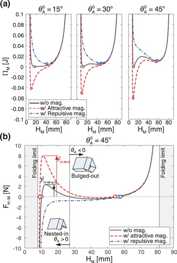
Figure 4. Effects of magnets on the SMO structure's stability profile and static characteristics. (a) Total potential energy landscapes of the structure corresponding to the no-magnet, the repulsive-magnet, and the attractive-magnet layouts. From the left to the right, the stress-free angle 
 and
and  (b) With
  the force–displacement relations corresponding to the no-magnet, the repulsive-magnet, and the attractive-magnet layouts. The stable configurations are denoted by empty circles; the critical forces for snap-through transitions from the nested-in to the bulged-out configuration are also marked.
Download figure:
Standard image High-resolution imageIn addition to controlling the number and positions of the stable configurations, the depths of the potential wells can also be effectively tailored. For example, attractive magnets can effectively deepen the depth of the potential well at the nested-in configuration. This will also affect the structure's static and dynamic characteristics.
The structure's force–displacement relation along the height direction can be obtained via

Figure 4(b) shows the constitutive relations corresponding to the no-magnet, the repulsive-magnet, and the attractive-magnet layouts, with the stress-free angle  The magnet-induced changes of the stability profile also transform the static characteristics. With repulsive magnets, the constitutive relation experience qualitative changes that the stable nested-in configuration and the negative stiffness segment are removed. The attractive magnets do not change the stability profile qualitatively; but quantitatively, the deepened potential well significantly raises the critical force level for a snap-through transition from the nested-in to the bulged-out configurations. Specifically, the critical force increases by more than two times from
  to
to  where the hat denotes the critical force, the subscript 'M' denotes the Miura-ori structure, 'w/o' and 'A' denote the no-magnet and the attractive magnet layouts, respectively.
3.4. Example 2: a magnetic-elastic coupled Kresling-ori structure
We then investigate the magnetic-elastic coupled Kresling-ori structure based on the design given in figure 2(f). Specifically, 8 magnets are embedded on the top-layer vertices, and 8 magnets are embedded in the bottom-layer side centers. Table 2 lists the geometric and physical parameters of the Kresling-ori structure and the used magnets (NdFeB, Grade N52). Substituting the geometric parameters into the constraint equations (6) and (7), the strain in the fold  (
( ) and the dihedral angles (
 and
and  ) can be determined for each rotation angle
  (figure 5(a)). Setting the open configuration as the stress-free state and based on the obtained dihedral angles, the total elastic potential energy can be determined via equation (16). Figure 5(b) displays the profiles of the total elastic potential energy as well as its constituents. It reveals that the elastic potential energy originating from the virtual folds (i.e. panel bending) account for the main parts, and the Kresling-ori structure is intrinsically bi-stable, with two potential wells (stable configurations) locating at
  and
and  We remark here that generally, owing to the contribution of panel bending, the elastic potential energy profile of the Kresling-ori structure is much higher than the Miura-ori structure (except when approaching the folding limits of Miura-ori). Therefore, multiple magnets (in this design example, 16 magnets) have to be integrated into the Kresling-ori structure to generate strong magnetic potential energy so that the inherent elastic potential energy profile can be significantly affected.
Table 2. Parameters of the magnetic-elastic coupled Kresling-ori structure.
| Parameters | Values | Parameters | Values |
|---|---|---|---|

|
8 |

|
0.8 N rad−1 |

|
30.00 mm |

|
6.35 mm |

|
0.98 |

|
6.35 mm |

|
8 mN rad−1 |

|
1.44 T |

Figure 5. Kinematics and elastic potential energy of the Kresling-ori structure based on the geometric parameters listed in table 2. (a) The strain in the fold  (
( ) and the dihedral angles (
 and
and  ) with respect to the rotation angle
  (b) Total elastic potential energy and its constituents with respect to the structure height
  where the two potential wells (corresponding to the two stable configurations) are marked by empty circles.
Download figure:
Standard image High-resolution imageTo conveniently examine the magnetic potential energy, the magnets in the top layer are numbered from '1' to '8', and the magnets in the bottom layer are numbered from '9' to '16'. Note that the relative positions among the magnets in the same layer remain immutable during folding; while for the magnets in different layers, their relative positions would experience significant changes, which would, therefore, alter the magnetic potential energy. Generally, the net force applied on the top-layer magnet 'j' ( j = 1, ..., 8) is the vector sum of the magnetic forces exerted by the bottom-layer magnets (with dipole moment
  i = 9, ..., 16 ) on the top-layer magnet j (with dipole moment
  ). Hence, based on equation (11), we have
Equation (18) is capable of capturing both the vertical and torsional components of the magnetic forces. Since all magnets are identical, aligned along the z-axis, and pointing in the z-direction, the corresponding magnetic dipole moment can be expressed as  For the repulsive-magnet layout, the top and bottom layer magnets take the opposite signs; for the attractive-magnet layout, they take the same sign. To vividly illustrate the above concept, as an example, figure 6(a) shows the magnetic force components exerted by the bottom layer magnets '9' to '16' on the top layer magnet '1' at a certain folded configuration. With respect to folding, the magnet '1' will experience a spatial translation, whose trajectory is given in figures 6(a) and (b). Along this trajectory, the magnitude of the net force applied on magnet '1' increases significantly as the height decreases, and its direction also undergoes noteworthy changes, as discretely depicted in figure 6(b).

Figure 6. Effects of magnets on the Kresling-ori structure's stability profile and static characteristics. (a) Magnetic force components exerted by the bottom-layer magnets on the top-layer magnet '1'. For clearness, other top-layer magnets are not shown. (b) Magnitudes of the net magnetic force applied on the top-layer magnet '1' with respect to the structure height; its direction changes along the translation trajectory are discretely depicted in the inset. (c) Total potential energy profiles of the structure corresponding to the no-magnet, the repulsive-magnet, and the attractive-magnet layouts. The potential energies originating from the repulsive and attractive magnets are also provided. (d) The force–displacement relations of the structure corresponding to the no-magnet, the repulsive-magnet, and the attractive-magnet layouts. The stable configurations are denoted by empty circles.
Download figure:
Standard image High-resolution imageAssuming zero magnetic potential energy at the open configuration and based on equation (18), the magnetic potential energy of the whole system can be expressed as

where  is the translation trajectory of magnet
  with respect to folding; it is a function of the structure height
  or the rotation angle
  Figure 6(c) displays the total potential energy of the Kresling-ori structure versus its height. Attaching magnets to the bi-stable Kresling-ori structure, the stable configuration at
  is little affected due to the weak magnetic forces. However, the stable configuration at
  experiences great changes. When the top-layer and bottom-layer magnets are attractive, the stable configuration at
  is moved to
  and the corresponding potential well is significantly depended. When the magnets are repulsive, in addition to a large translation of the stable configuration from
  to
to  the configuration at
  becomes stable, i.e. the stability profile of the structure undergoes a qualitative change from bi-stable to tri-stable. Similarly, based on
  the structure's constitutive force–displacement relations corresponding to the no-magnet, the repulsive-magnet, and the attractive-magnet layouts can be obtained (figure 6(d)).
The above two examples vividly demonstrate the effects of magnets in controlling origami structures' stability profile as well as the corresponding static characteristics. Quantitatively, the magnets could translate the potential well (i.e. the stable configuration), deepen or shallows the potential well (i.e. alter its stability degree). Qualitatively, the magnets could eliminate the original stable configuration or add additional stable configuration to the structure. These changes would thus fundamentally alter the structure's constitutive force–displacement relations. We point out here again that if replacing the permanent magnets with electromagnets, such tailoring could be achieved more easily by controlling the electric currents.
4. Prototypes and experimental verification
To verify the predicted effects of incorporating magnets, proof-of-concept prototypes are fabricated and tested. Evolutions of origami structures' stability profiles are evaluated via the experimental force–displacement relations.
4.1. Magnetic-elastic coupled Miura-ori structure prototype
Figures 7(a) and (b) show the design and prototype of the magnetic-elastic coupled Miura-ori structure based on the parameters given in table 1. The origami facets are water jet cut individually from 0.25 mm thickness austenitic stainless-steel sheets. Note that austenitic stainless steels can be classed as paramagnetic with relative permeabilities approaching 1.0 (generally in the range between 1.003 and 1.05 in the fully annealed condition). Such low permeabilities enable austenitic steels to be used as 'non-magnetic' materials, with their effects on the magnetic field being negligible. To prevent possible contacts between the facets and the top/bottom magnets, part of the facets around the vertex are cut out. These facets are pasted to a 0.13 mm thickness adhesive-back plastic film (ultrahigh molecular weight polyethylene) to form individual Miura-ori cells. The two cells are then connected along the connecting creases by adhesive-back films to form an SMO structure. Through this construction, the steel facets are significantly stiffer than the plastic creases to ensure rigid-foldability. In addition, we paste 0.1 mm thickness pre-bent spring-steel stripes at the folds of the top cell to provide strong torsional stiffness (i.e. a high  ), thus imparting bi-stability to the SMO structure. To install the SMO structure on the universal testing machine, 3D-printed connectors are screwed to rectangular connection plates, which further connect with the SMO cell at the top and bottom creases through adhesive-back films. To ensure free rotation of the SMO structure as well as effective load transmission during compression/tension tests, non-magnetic ball bearings are embedded into embedded into the connectors, and a non-magnetic titanium screw rod is inserted through the bearing, with one end fixing with the 3D-printed magnet holder, and the other end fixing with the universal testing machine. Here, NdFeB magnets (see parameters listed in table 1) are employed for proof-of-concept experiments.

Figure 7. Experiments on the magnetic-elastic coupled Miura-ori structure prototype. (a) Design of the prototype. (b) Photo of the prototype assembled on the universal testing machine. (c) Measured force–displacement curves of the prototype corresponding to the no-magnet, the attractive-magnet, and the repulsive-magnet layouts. The curves denote the measured averages, and the shaded bands denote the standard deviations. The stable configurations (empty circles) and the critical forces for snap-through switches are indicated. Insets show the photos of the prototype during folding.
Download figure:
Standard image High-resolution imageTo experimentally verify the effects of magnets, displacement-controlled compression and tension tests are carried out on the prototypes with the no-magnet, the repulsive-magnet, and the attractive-magnet layouts, respectively. Figure 7(c) shows the measured force–displacement relations corresponding to the three layouts. For each layout, five complete quasi-static tension and compression tests (with speed 10 mm min−1) are performed; for each test, we average the tension and compression test data to get one curve. Averaging the five curves yields the measured average (the curves) and the standard deviations (shaded bands). Figure 7(c) reveals that when there is no magnet, the prototype exhibits bi-stability. By integrating repulsive magnets, the original bi-stable profile is altered to mono-stable, where the stable bulged-out configuration remains stable, while the nested-in configuration is no longer stable. By integrating attractive magnets, although the prototype remains bi-stable, the stable nested-in configuration is significantly translated, and the critical force for the snap-through switch is remarkably lifted. Therefore, in terms of the qualitative characteristics, the experimental curves are in good agreement with the theoretical predictions displayed in figure 4(b).
It is worth pointing out that in the experiment, when the prototype is compressed toward its lower kinematic folding limit, the distance between the two attractive magnets (i.e.  ) becomes very small, and the magnetic force becomes extremely strong to possibly damage the prototype. In detail, experimental trials reveal that the strong magnetic attraction would deform the steel facets, tear the adhesive film, and let the two magnets stick together. To prevent such a scenario and to ensure safety, the compression tests are manually stopped when a force fall is detected. Such a procedure does not affect the identification of qualitative characteristics.
4.2. Magnetic-elastic coupled Kresling-ori structure prototype
Figures 8(a) and (b) show the design and prototype of the magnetic-elastic coupled Kresling-ori structure based on the parameters given in table 2. The origami structure is made of 0.076-mm-thickness moisture-resistant polyester film. We use laser-based machining techniques to cut and pattern flat sheet. Specifically, the creases are perforated to some extent such that the bending stiffness of the creases is weakened; we also cut small holes at the vertices where multiple creases intersect to prevent stress concentration. Through folding, rolling, and gluing, a Kresling-ori structure can be obtained. To embed magnets and to connect with the universal testing machine, the Kresling-ori structure is connected with two acrylic plates at the top and bottom. Note that during folding, the top plate would rotate with respect to the bottom plate. To ensure free rotation, similarly, ball bearings are embedded into the 3D-printed connectors, which further connect with the top and bottom acrylic plates. A non-magnetic titanium screw rod is inserted through the bearing, with one end fixing with the plate, and the other end fixing with the universal testing machine. Here, NdFeB magnets (see parameters listed in table 2) are employed for proof-of-concept experiments.

Figure 8. Experiments on the magnetic-elastic coupled Kresling-ori structure prototype. (a) Design of the prototype. (b) Photo of the prototype assembled on the universal testing machine. (c) Measured force–displacement curves of the prototype corresponding to the no-magnet, the attractive, and the repulsive magnet layouts. The curves denote the measured averages, and the shaded bands denote the standard deviations; the stable configurations are also indicated by empty circles. (d) Configurations of the prototype during tests.
Download figure:
Standard image High-resolution imageDisplacement-controlled compression and tension tests are carried out on the prototype for the no-magnet, the attractive-magnet, and repulsive-magnet layouts, respectively. Based on the same testing and data processing procedures as we used in subsection 4.1, figure 8(c) shows the measured force–displacement relations of the magnetic-elastic coupled Kresling-ori prototype corresponding to the three layouts. It reveals that when there is no magnet, the prototype is bi-stable (figure 8(c), left). By integrating attractive magnets, the structure's constitutive relation evolves into a mono-stable profile (figure 8(c), middle), which, however, contradicts with the theoretical prediction (which is a bi-stable profile, shown in figure 6(d), dashed). Carefully observing the curves and the prototype's deformation during folding, the attractive magnets have little effects on the first half of the curve and the stable 'open' configuration; with the height decreasing, large discrepancies occur, which are induced by two reasons. First, in theoretical analysis, the origami panels are assumed to be rigid, which are strong enough to drag the magnets so that their configurations exactly follow the folding kinematics. Based on such assumptions, the overall reaction force of the prototype will experience an inflection point from declining to increasing, generating a stable 'close' configuration (see the dashed curve in figure 6(d) and the dashed curve in figure 8(c), middle). However, in experiments, when the prototype is compressed to a relatively small height, the attractive force between the top-layer and the bottom-layer magnets becomes so strong that the origami panels made of thin polyester films are no longer able to drag the magnets following the folding kinematics. Hence, when the prototype is further compressed, although the top-layer magnets will gradually decline, their lateral positions with respect to the bottom-layer magnets will be locked. In this process, the polyester-film panels will be seriously deformed; however, due to the increasingly strong magnetic attraction, the overall reaction force of the prototype keeps negative and declines fast, giving rise to a mono-stable profile. Second, theoretical analysis assumes zero-thickness of the facets and creases, but practically, when the prototype is compressed into small height, the film thickness cannot be ignored anymore. The films will be contacted and pressed seriously, which generate significant elastic force that would affect the overall profile. This explains why the reaction force starts to increase when the prototype is compressed to below 
By integrating repulsive magnets, the original bi-stable profile evolves into tri-stable (figure 8(c), right), where the stable 'open' configuration remains stable, while the stable 'closed' configuration is translated to a configuration with larger height. Keep compressing the prototype beyond the stable 'closed' configuration, the reaction force increases again, and then experiences a sudden drop, suggesting a snap-through transition of the configuration. Theoretically, such drop will continue until the test ends, and the final configuration would be an additional stable state brought by the repulsive magnets (see figure 6(d)). However, in experiments, the sudden force drop is followed by a fluctuating interval, and then the force rises again until the end. Such discrepancies between the theoretical and experimental results are also caused by the non-ignorable material thickness of the prototype. When the prototype is compressed into small height, the films will be contacted and pressed, which therefore interrupts the configuration snap-through and increases the reaction force undesirably. Particularly, at the final stage of the test, the film compressions become significant, which will increase the reaction force.
In short, based on proof-of-concept prototypes of Miura-ori and Kresling-ori structures, the effects of magnets on the stability profiles and the force–displacement constitutive relations are verified, which includes qualitative transitions (switches among mono-stable, bi-stable, and tri-stable) and quantitative evolutions (translations of the stable configurations, deepening or shallowing of the potential wells). Due to the deformation and inter-pressing of the polyether-film panels, non-negligible discrepancies are observed when testing the magnetic-elastic coupled Kresling-ori prototype; this triggers an interesting research problem that has not been tackled, that is, what is the effects of magnet-origami integration when the origami panels and creases are flexible to exhibit large deformations.
5. Dynamics
Changes of the stability profile and the corresponding force–displacement relation would, in turn, affect the structure's dynamic characteristics; this will be particularly significant if such changes are qualitative. This section numerically studies the effects of magnets on the system dynamics of an example magnetic-elastic coupled Miura-ori structure.
5.1. Simplified system and equation of motion
Figure 9(a) schematically displays the setup for dynamic study. Specifically, the magnetic-elastic coupled Miura-ori structure is horizontally suspended on a fixed frame with light strings. A lumped mass  connects with the origami structure at one end, and harmonic base excitations are applied on the structure at the other end. Here, the lumped mass is assumed to be much heavier than the origami structure, such that the origami can be equivalently considered as a massless nonlinear spring with force–displacement relation
  and a massless viscous damper with damping coefficient
  Thus, the system in figure 9(a) can be simplified into a spring-lumped-mass model (figure 9(b)), with
  and
and  denoting the absolute displacements of the lumped mass and the base, respectively, and
  denoting and the relative displacement between the lumped mass and the base. The origin of the relative displacement (i.e.
  ) is set at the unstable equilibrium of the SMO structure without magnet. Based on the example shown in figure 4(b) (with parameters listed in table 1, and
  ), the
  configuration is set at
  Hence, the equation of the motion of the equivalent model yields

where the dots over the variables denote time derivatives. The base is subjected to harmonic excitation  with amplitude
  and frequency

Figure 9. Dynamic study on the magnetic-elastic coupled Miura-ori structure. (a) Setup for dynamic study. (b) The equivalent model of the system. (c) The analytical and fitted force–displacement relations corresponding to the no-magnet, the repulsive-magnet, and the attractive-magnet layouts.
Download figure:
Standard image High-resolution imageNote that the constituent force–displacement relations of the magnetic-elastic coupled Miura-ori structure possess strong nonlinearity originating from the origami geometry and the magnetic effect. For the sake of convenience in numerical studies, the constitutive relations corresponding to the no-magnet, the repulsive-magnet, and the attractive-magnet layouts are fitted with polynomials up to 27th orders, respectively. Figure 9(c) displays the theoretical and the fitted curves of the three constitutive relations, which are in good agreement; particularly, the stable and unstable equilibria of the system are well captured. Note that as expected, some undesired small fluctuations exist, and when  approaches to the folding limits, the fitted relations cannot fully reflect the kinematic constraints. However, such fittings would still be effective in demonstrating the effects of magnets on dynamics.
5.2. Numerical analyses
The following parameters are assigned for numerical analyses: 
 and
and  Based on the fitted force–displacement relations corresponding to the no-magnet, the repulsive-magnet, and the attractive-magnet layouts, equation (20) is solved via the 4th-order Runge–Kutta method with zero initial condition, i.e.
  respectively. With a step of 0.1 Hz, a discrete frequency sweep is performed between 2 and 20 Hz. With a fixed displacement excitation amplitude
  the higher the excitation frequency, the larger the input energy. At each frequency, the simulation time is long enough to let the system enter steady-state. The peak-to-peak value of the relative displacement (
 ) and the system's displacement transmissibility in terms of the root-mean-square (RMS) value (specifically,
  ) are examined to uncover the system's dominant dynamic behaviors. Specifically,
  is defined as
where  and
and  (
( ) are numerical sampling points in the steady-state displacement-time histories of the lumped mass and the base, respectively.
Figure 10 displays the dynamic responses of the magnetic-elastic coupled origami structure corresponding to the three layouts. When there is no magnet applied, the structure is inherently bi-stable (refer to figure 4). Under external excitations, three qualitatively different types of responses can be observed: intra-well (in) oscillations that surround the nested-in stable configuration, intra-well (out) oscillations that surround the bulged-out stable configuration, and large-amplitude inter-well oscillations that surround the two stable configurations (figure 10(a)). They present distinctly different displacement transmissibility levels. When the excitation frequency is relatively low, the structure could exhibit both intra-well (in) and intra-well (out) oscillations. Note that due to the low energy barrier between the nested-in and the bulged-out stable configurations (refer to figure 4), transitions from the intra-well (in) oscillations to the intra-well (out) oscillations occur at very low frequency (2.3 Hz). By increasing the excitation frequency, the input energy becomes large enough to maintain inter-well oscillations, which continue appearing above 8.6 Hz.

Figure 10. Dynamic responses of the magnetic-elastic coupled Miura-ori structure corresponding to (a) the no-magnet layout, (b) the attractive-magnet layout, and (c) the repulsive-magnet layout. The top row displays the peak-to-peak values of the relative displacement ( ) with respect to the excitation frequency, where the structure's stable configurations are denoted by the dashed horizontal lines; the bottom row displays the displacement transmissibility in terms of the RMS value with respect to the excitation frequency.
Download figure:
Standard image High-resolution image
When attractive magnets are applied, the structure remains bi-stable. Similarly, three types of responses with distinct displacement transmissibility levels are observed, namely, intra-well (in) oscillations, intra-well (out) oscillations, and inter-well oscillations (figure 10(b)). However, with the attractive magnets, the potential well at the nested-in configuration is significantly deepened, which raises the energy barrier from the nested-in to the bulged-out stable configurations, and correspondingly, increases the critical force for snapping through to the bulged-out configuration (refer to figure 4). Hence, when the excitation frequency is relatively low, the input energy is insufficient to overcome the potential energy barrier, and the structure sustains at intra-well (in) oscillations. By increasing the excitation frequency to 6.5 and 6.6 Hz, inter-well oscillation and a transition to the intra-well (out) oscillation are observed for the first time. When the excitation frequency is further increased to 11.4 Hz, the input energy becomes sufficient to maintain large-amplitude inter-well oscillations. Comparing to the no-magnet layout, the critical frequency for transiting from intra-well (in) oscillations to intra-well (out) oscillations and the critical frequency for exhibiting persistent inter-well oscillations are significantly increased.
When repulsive magnets are applied, the structure turns into mono-stable (refer to figure 4), which fundamentally alter the system's dynamic responses (figure 10(c)). Overall, the frequency-response diagram shows representative characteristics of hardening nonlinearity. In detail, unlike the bi-stable scenarios that the oscillations surround different stable equilibria, here, basically, the structure is able to output two types of responses (namely, high-amplitude responses and low-amplitude responses) that surround the same stable equilibrium but are different in the amplitude level and the displacement transmissibility level. Note that some complex dynamic behaviors (e.g. responses with subharmonic components) are also observed, which also surround the only stable equilibrium.
It's worth mentioning here that with only one pair of initial conditions, the system's dynamics cannot be fully captured; this is because the structure possesses strong global nonlinearity such that its responses are extremely sensitive to initial conditions [44]. Carrying out a comprehensive dynamic analysis of the structure by considering the nonlinearities originating from the origami geometry and the magnets is an interesting topic to be explored.
In short, by numerically examining the dynamic responses of the magnetic-elastic coupled Miura-ori structure, the effects of the attractive and repulsive magnets on system dynamics are exemplified. The attractive magnets could quantitatively change the critical frequency for transiting intra-well (in) oscillations to intra-well (out) oscillations and the critical frequency for exhibiting continuous inter-well oscillations; the repulsive magnets could qualitatively switch the structure's dominant dynamic characteristics from bi-stability to hardening nonlinearity. Such qualitative and quantitative changes on dynamics suggest the possibility and feasibility of using magnets to control origami structures' dynamic responses, and hence, to harness their dynamic functionalities.
6. Summaries and conclusions
Multi-stable mechanical metamaterials and structures are capable of exhibiting different mechanical properties and outputting distinct dynamic responses at different stable configurations. For these peculiar merits, they have received considerable research attention in many domains. Particularly, origami, the art of paper folding, featuring with extraordinary capabilities in constructing and deforming 3D shapes, has provided novel inspiration, elaborate 3D configuration, and infinite design space to the development of multi-stable origami structures. Although possessing marked advantages originating from folding, the further development of multi-stable origami structures is faced with a tremendous demand for acquiring tunability of the stability profile and adaptability of mechanical properties. This research, as a result, makes a significant and beneficial attempt by employing magnets to quantitatively and qualitatively alter the structure's potential energy landscape, thus achieving tunability of the stability profile. Quantitative changes include translations of the potential wells, deepening and shallowing of the potential wells; qualitative changes manifest as the switches of the profile among mono-stability, bi-stability, and tri-stability. Through two examples, the magnetic-elastic coupled Miura-ori structure and the magnetic-elastic coupled Kresling-ori structure, we observed that the stability profile changes could further affect the structures' mechanical properties, e.g. fundamentally alter the structures' constitutive force–displacement relation. Based on proof-of-concept magneto-origami structure prototypes with permanent magnets, the predicted magnet-induced effects are verified. The investigation is also extended to the dynamics realm, motivated by the facts that origami structures will be inevitably working in a dynamic environment or under dynamic excitations. Numerical analyses reveal that the quantitative changes of the stability profile could translate the critical frequencies for switching dynamic responses, and the qualitative changes of the stability profile could fundamentally alter the frequency-response relations.
Overall, by revealing the magnet-induced evolutions of the origami structure' static and dynamic characteristics, this research could significantly advance the state of the art of the development of multi-stable metamaterials and structures that are inspired by origami. The proposed magnet-based innovation could effectively endow the origami structures with the long-desired tunability of the stability profile and mechanical properties, making them attractive in applications that call for adaptabilities, such as adjustable shape morphing and broadband energy harvesting.
Through the above theoretical, numerical, and experimental studies, we also recognize many interesting issues that worth further investigation to systematize the magnet-based approach. For example, since electromagnets could effectively and efficiently change the magnetic field strength as well as reverse the pole layout, it would be very interesting and necessary to design new prototypes based on electromagnets to achieve on-line tunability. The magnetic effect and the origami geometry introduce significant nonlinearities into the structure, it is therefore imperative to perform comprehensive dynamic analyses to systematically uncover the magnet-induced switches of nonlinear dynamic behaviors. The behavior of magneto-origami structures will be significantly complex if the origami structures are flexible or soft; this constitutes a challenging research topic because of the difficulty in modeling and analyzing soft origami structures. The size of magnets is always non-negligible that may affect the folding of the origami structure, which calls for integrated design and prototyping by putting the magnet size into consideration.
Acknowledgments
This research was supported by the National Natural Science Foundation of China under award No. 11902078 and No. 91748203, the US National Science Foundation under award No. 1634545, and the University of Michigan Collegiate Professorship.