
Abstract
Vibration energy harvesters (VEHs) offer an alternative to batteries for the autonomous operation of low-power electronics. Understanding the influence of scaling on VEHs is of great importance in the design of reduced scale harvesters. The nonlinear harvesters investigated here employ velocity amplification, a technique used to increase velocity through impacts, to improve the power output of multiple-degree-of-freedom VEHs, compared to linear resonators. Such harvesters, employing electromagnetic induction, are referred to as velocity amplified electromagnetic generators (VAEGs), with gains in power achieved by increasing the relative velocity between the magnet and coil in the transducer. The influence of scaling on a nonlinear 2-DoF VAEG is presented. Due to the increased complexity of VAEGs, compared to linear systems, linear scaling theory cannot be directly applied to VAEGs. Therefore, a detailed nonlinear scaling method is utilised. Experimental and numerical methods are employed. This nonlinear scaling method can be used for analysing the scaling behaviour of all nonlinear electromagnetic VEHs. It is demonstrated that the electromagnetic coupling coefficient degrades more rapidly with scale for systems with larger displacement amplitudes, meaning that systems operating at low frequencies will scale poorly compared to those operating at higher frequencies. The load power of the 2-DoF VAEG is predicted to scale as  (s = volume1/3), suggesting that achieving high power densities in a VAEG with low device volume is extremely challenging.
Export citation and abstract BibTeX RIS
1. Introduction
Recent advancements in low-power electronics have increased the deployment of wireless sensor networks (WSNs) for the pervasive monitoring of environmental conditions. WSNs consist of distributed networks of static sensor nodes, which have evolved such that they can operate effectively at extremely low-power levels [1]. This technology has a vast range of applications, including human and structural health monitoring, building energy management, and monitoring of transportation systems [2]. Contemporary sensor nodes rely on battery technology for power; batteries, however, suffer from multiple issues, foremost among them being their finite operational lifetime and environmental impact [3]. Vibration energy harvesting technologies seek to scavenge ambient vibrational energy to supplement or replace batteries for the unlimited autonomous powering of sensor nodes [4].
Ambient vibrational energy is pervasive, with potential sources for small-scale power generation including industrial machinery, transportation systems and human motion [5]. As such, in the last two decades, vibration energy harvesters (VEHs) have been the subject of significant research. VEHs, which are typically spring-mass-dampers, extract mechanical energy from a vibrating source and convert it into useful electrical energy. This can be achieved through a number of transduction mechanisms, with electromagnetic induction—based on Faraday's law—of interest herein.
The majority of research into VEHs initially was focused on linear VEHs, which allow energy to be harvested at a narrow frequency range corresponding to the resonant frequency of the linear spring-mass-damper [6–8]. The spectra of ambient vibrations, however, are often temporally varying, broadband, or random in nature. Consequently, a broadband energy harvester, which can harvest energy over a range of frequencies, is desirable.
A number of broadband energy harvesting techniques have been developed to increase the effective operational frequency range of VEHs, namely frequency tuning [9, 10], multi-modal [11, 12], and nonlinear methods [13, 14]. Nonlinear methods also include piecewise linear (PWL) oscillators [15, 16], which typically employ impacts with end stops to achieve a discontinuous stiffness.
The energy harvesters under investigation are referred to as velocity amplified electromagnetic generators (VAEGs). These devices utilise impacts to enhance the performance of multiple-degree-of-freedom (multi-DoF) electromagnetic generators by increasing the relative velocity between the transducer components (magnet and coil). In comparison with the PWL harvesters employing impacts with end stops, the VAEGs described herein achieve this naturally through their geometry and configuration of masses. The VAEGs utilise free-moving masses and, hence, do not require anchored springs. This is beneficial as there is no spring force acting against the masses, allowing ballistic motion and higher velocities to be achieved.
Velocity amplification in VEHs was first employed by [17]. VAEGs with 2- and 3-degrees-of-freedom (DoF) were tested against a single-DoF system, with the multi-DoF systems offering an improvement in power generation. More recently [18], investigated different implementations of 2-DoF VAEGs [19], utilised magnetic springs in a 2-DoF VAEG to achieve a high power output at relatively low frequencies, and [20] developed a 2-DoF VAEG which employed a triboelectric nano-generator. The influence of mass ratio and number of DoFs on the velocity and voltage output of VAEGs was investigated by [21]. It was determined that under forced excitation, contrary to velocity amplification theory, the highest RMS velocity of the smallest mass is achieved by a 2-DoF VAEG. This is because the more complex impact sequences which occur in the higher DoF systems result in lower RMS velocities. Consequently, the VAEGs implemented in this investigation are 2-DoF systems. It was also demonstrated that velocity amplification increases with mass ratio—the ratio of the largest to the smallest mass in the system—resulting in higher RMS velocities. Increasing mass ratio reduces the size of the final mass, however, which limits the possible size of the magnet within the final mass. As a consequence, the output voltage does not increase with mass ratio, despite the increase in RMS velocity. The conclusion of the investigation into the influence of mass configuration is that VAEGs with 2-DoFs and low mass ratios are the optimal VAEG configuration.
As a result of the investigation into the influence of mass configuration on VAEGs [21], a 2-DoF VAEG with mass ratio R = 3 is investigated, through experimental and numerical methods. The harvester design and model are described in section 3, while section 4 presents the experimental set-up employed. In section 5, the system is characterised for a range of input excitation conditions, as well as for changing gap length—a key geometric parameter that influences the device behaviour. This characterisation is of importance as it demonstrates the changing behaviour of the 2-DoF VAEG system with varying excitation conditions and geometric configurations, which has not previously been shown.
In section 6, an investigation into the influence of scaling on VAEGs is undertaken. It is of great importance to understand the influence of scaling on electromagnetic VEHs in the development of reduced scale harvesters. Reflecting this importance, the effect of scaling on linear electromagnetic harvesters has been well documented in the literature [22–26]. However, due to the greater complexity of nonlinear VAEGs, relative to linear harvesters, linear scaling theory cannot be directly applied to VAEGs. Hence, there is a need for a method of nonlinear scaling analysis. This method is developed and employed here to perform a scaling analysis of 2-DoF VAEGs. Mathematical models of the system are solved numerically to show the influence of scaling, with the models validated through experimentation.
2. Velocity amplification
The velocity amplification effect is realised through sequential impacts between free-moving masses of decreasing size, resulting in a velocity increase of the lighter mass according to the conservation of momentum (a detailed description of velocity amplification theory was presented in a previous publication by O'Donoghue et al [21]). For electromagnetic generators, an increase in power generation is achieved by increasing the relative velocity between the coil and magnetic field,  , as the power generated is proportional to the relative velocity squared (
 ). Velocity amplification can be employed in multiple-DoF VEHs by coupling the masses to a transducer. Herein, the final mass in the stacked mass system, which is magnetically active, oscillates axially relative to a coil attached to the harvester base. The masses are vertically stacked and free-moving, with springs interposed between the masses to achieve high restitution impacts.
The mass ratio, R, between the masses in a velocity amplified system is given as the ratio of the initial largest mass, m1, to the final smallest mass, mn. For the 2-DoF systems discussed here, this reduces to:

3. 2-DoF VAEG
The 2-DoF VAEG design and its model are described in this section.
3.1. Harvester design
The VAEG under investigation was a 2-DoF VAEG with a mass ratio of R = 3. The device was fabricated at three scales and underwent homothetic scaling, i.e. it was uniformly scaled. As such, a number of the design decisions implemented were based on the use of the prototype for the scaling analysis, presented in section 6. The mid-scale prototype is shown in figure 1. The design of the 2-DoF VAEG at the three scales is discussed below:
- (a)Active components and support structure
- The 2-DoF VAEG consisted of a copper base mass and a lighter magnet stack. It was designed such that both the copper mass and the magnet stack oscillated within a cylindrical Teflon tube. Copper was selected for the base mass because of its high density and non-magnetic properties.
- The support structure of the harvester (figure 1(a)) was able to accommodate the three prototype scales, as the Teflon tubes were able to be inserted into the base and cap, and then fixed in place.
- The interior of the tube is shown in figure 1(b), with the masses in their rest positions. Both masses were disconnected from the springs and were able to move freely along the inside of the Teflon tube. The springs were non-magnetic stainless steel compression springs, with the spring stiffness at each scale chosen, such that the natural frequency of an equivalent linear system would remain constant.
- For the transducer, magnet diameters of dmag = 12, 8 and 6 mm were chosen (figure 1 features the dmag = 8 mm harvester). As the volume scales with the cube of the dimension and uniform scaling was employed, the resultant transducer volumes, normalised to the volume of the largest magnet stack were 1, 0.296 and 0.125. The transducer arrangement is discussed in further detail in 3.2.3.
- (b)Adjustable parameters.
- The gap length, g0, (figure 1(b)) is the distance through which the masses can travel free from any spring force. Adjusting g0 has a significant effect on the dynamics of VAEGs (discussed in section 5). In the 2-DoF VAEG presented here, g0 was adjusted by changing the cap position. Two slots along the length of the top of the tube allowed the cap position to be raised or lowered along the Teflon tube and stainless steel shafts.
- The coil holder was designed to be adjustable—by sliding along the shafts external to the Teflon tube—as the optimal position of the coil relative to the magnet stack varied with g0. Set screws were used to hold the cap and coil holder in place.
- (c)Mechanical damping considerations—minimising mechanical damping to maximise the power generation.
- The copper mass was designed to reduce friction with the Teflon wall. Three ridges along the length of the mass limited the surface area of the copper in contact with the tube, reducing friction.
- The same design was employed in the Teflon caps attached to the magnet stack.
- An air-release gap was present at the base of the Teflon tube to reduce squeeze-film damping effects.
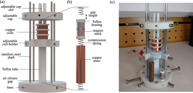
Figure 1. (a) Model of the mid-scale harvester and support structure, (b) tube inner structure showing active components, and (c) the fabricated VAEG.
Download figure:
Standard image High-resolution image3.2. System model
To model a VAEG, it is necessary to develop equations of motion and a further equation for the electrical system.
3.2.1. Dynamical system
The VAEGs discussed herein utilise impacts in free-moving masses to achieve velocity amplification, as described in section 2. Each mass can, therefore, be forced upon by a spring or can be free of any spring force, resulting in piecewise-linearity. PWL systems have received significant investigation in the field of nonlinear dynamics [27–29]. Piecewise linearity arising from impacts has also been investigated to improve the performance of VEHs in systems referred to as impact oscillators [18, 30–32].
The 2-DoF VAEGs presented here are modelled as PWL inertial oscillators. A schematic of a 2-DoF PWL system is shown in figure 2. The springs do not transfer load in tension, meaning that the masses can become detached from the springs.
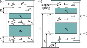
Figure 2. Schematic of a 2-DoF PWL harvester; (a) m1 and m2 at positions z1 = 0 and z2 = 0, respectively, with springs and dampers; (b) displaced masses detached from springs, showing base (y(t)), absolute (x1,2), and relative (z1,2) displacement.
Download figure:
Standard image High-resolution imageThe transducer is coupled between m2 and the base. This involves incorporating a magnet in m2, with a coil that is attached to the device housing arranged concentrically to the mass. Therefore, the electrical damping force,  , is applied in the equation of motion of m2 only. As shown by (7), the electrical damping force can also be written as Ki.
As this is a 2-DoF system, there are two equations of motion, which are determined by applying a force balance to each of the masses. The masses are considered to be point masses in the model; therefore, their height is zero. The relative displacements of the masses and the base are  and
and  , while the relative velocities are then
  and
and  . Considering the 2-DoF system as a PWL oscillator with detachable masses, the stiffness and damping forces are discontinuous. Boundary conditions determine the forces acting on the masses at any instant:
- the base mass m1 is attached to the spring k1 under the condition z1 < 0;
- the two masses are attached to each other through k2 if z2 < z1; and
- m2 is in contact with the stopper spring k3 under the condition z2 > g0.
The set of coupled equations describing the dynamics of a 2-DoF PWL system are then:
3.2.2. Electrical system
When a conductor experiences a change in magnetic field, a voltage, Vind, is induced, which is equal to the temporal rate of change of magnetic flux, ϕ (Faraday's law). This can be rewritten as the product of the magnetic flux gradient and the relative velocity between the coil and magnetic field:

The flux gradient, often termed as the coupling coefficient, K, is the link between the mechanical and electrical domains:

where Br is the average radial magnetic flux density and lw is the total coil length. Substituting (5) into (4) gives a new expression for the induced voltage:

The movement of the coil through the magnetic field also results in an electrical damping force known as the Lorentz force:

where i is the current.
The electrical circuit of the VAEG implemented here consists of a generator connected in series with a coil resistance RC, load resistance RL, and coil inductance LC (figure 3(a)). Applying Kirchhoff's voltage law to the circuit:

where i is current. The coil resistance is given by:
where ρc is the resistivity of copper, and Aw is the coil wire cross sectional area. The coil inductance (in μH) is calculated using the Wheeler approximation [33]:
where the mean coil radius  , N is the number of coil turns, ctax is the coil thickness in the axial direction, and ctrad is the coil thickness in the radial direction (figure 3(b)). Rearranging (8) and substituting i = VL/RL (Ohm's Law) results in an equation for the load voltage:

This electrical circuit equation (11) is coupled to the equations of motion, (2) and (3), to model both the mechanical and electrical systems of the VAEGs. This system of equations is solved numerically by the MATLAB numerical ODE solver ode15s. It is necessary to use this solver (rather than a nonstiff solver such as ode45), as the set of coupled equations is stiff, i.e. the equations contain terms which rapidly change during the solution, potentially making the nonstiff numerical method of solving the equations unstable.
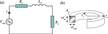
Figure 3. (a) Electrical circuit representation of an electromagnetic generator, and (b) multi-turn coil showing the geometric properties of the coil.
Download figure:
Standard image High-resolution image3.2.3. Modelling the coupling coefficient
For simplicity, the coupling coefficient, K, is often assumed to be constant in the analysis of electromagnetic energy harvesters. This assumption is valid if the displacement of the inertial mass is small. VAEGs, however, exhibit relatively large displacements. Therefore, to accurately model a VAEG, a coupling coefficient that varies with axial displacement, K(z), is necessary.
The transducer employed in the VAEG is illustrated in figure 4(a). The magnet stack consists of two oppositely polarised magnets with a soft magnetic spacer between them. The spacer acts as a flux concentrator to increase the radial flux at the centre of the magnet stack. The three individual coils are located at the regions of high radial flux density and are connected such that voltage cancellation is avoided. The process used to determine K(z) for the transducer employed here is outlined below.
- The static magnetic field of the permanent magnet stack was modelled using COMSOL multi-physics, the finite element analysis software, through the AC/DC module with the magnetic fields, no currents physics. The geometry of the magnet stack was defined in two dimensions about a central axis of symmetry with a surrounding air domain. The air domain was made sufficiently large (10× the magnet stack height and 10× the magnet stack diameter) such that the boundary condition on the exterior boundaries had a negligible effect on the field in the region surrounding the magnet. The magnet geometry and a portion of the surrounding air domain is illustrated in figure 5. The zero magnetic scalar potential condition was applied to the external boundaries in the model (the top, right and bottom sides of figure 5), while the magnetic insulation condition was applied to the axis of symmetry (the left side of figure 5). The model required the residual flux density, Bres, and magnet orientation as input parameters, with the model output being the radial magnetic flux density, Br—this is the radial component of the normal magnetic flux density shown in figure 5. To get an accurate calculation of the magnetic field, the model mesh (free tetrahedral) was refined until the magnetic flux density no longer changed with reduced mesh size.
- The average radial magnetic flux density,
 , in the axial direction—averaged across the coil width in the radial direction—is shown in figure 4(b).
 - K(z) is then the product of over the total coil length, lw (5). This was calculated for a range of coil positions relative to the magnet. A function was fitted to the result such that K(z) could be determined for any relative coil-magnet position (figure 4(c)).


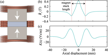
Figure 4. (a) Transducer configuration. (b) Average radial flux,  , along the axial direction at coil location. (c) Coupling coefficient K for varying coil positions relative to the magnet.
Download figure:
Standard image High-resolution image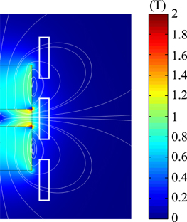
Figure 5. Flux distribution and density for the right half of the magnet stack with surrounding air domain. The coil locations implemented to find K(z) in figure 4(c) are shown as white rectangles.
Download figure:
Standard image High-resolution image4. Experimental set-up and method
The VAEGs were tested under sinusoidal forced excitation. A schematic of the experimental set-up is illustrated in figure 6. The system under test was mounted on the head of the V406 shaker. The shaker excited the system sinusoidally at the desired acceleration, with both single frequency and frequency sweeps employed. This was controlled by a Dactron Comet shaker control system. A high sensitivity (508 mV g−1) PCB Piezotronics accelerometer mounted on the shaker head measured the acceleration of the shaker, with the output signal providing feedback to the controller. A laser Doppler vibrometer (LDV) was also employed in this set-up to measure the velocity of the magnet stack under forced excitation. Measuring the output from the electrical system involved attaching the coil to a load of a known resistance value. The voltage generated in the coil was then recorded across this load resistor using LabVIEW.
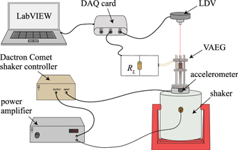
Figure 6. Schematic of the experimental set-up used in forced excitation tests for voltage and velocity measurements—Dactron Comet shaker control system employed.
Download figure:
Standard image High-resolution image5. 2-DoF VAEG characterisation
The characterisation of the 2-DoF VAEG is described in this section. Frequency sweeps at a range of acceleration levels and gap lengths are presented, with the results achieved compared to the best performing electromagnetic energy harvesters from the literature.
5.1. Characterisation sweeps
The device used in the characterisation tests was the dmag = 8 mm scale harvester. The system was tested experimentally using continuous frequency sweeps with the experimental set-up described in section 4. The frequency was swept from 6 to 45 Hz at a linear rate of 0.073 3 Hz s−1, giving a total sweep time of 531.8 s. The cap height was varied to achieve gap lengths (figure 1) of g0 = −0.2, 2.5 and 10.5 mm—the gap lengths were chosen to effectively demonstrate the range of responses shown by the device. These three configurations were tested at base acceleration levels ranging from Acc = 2–10 m s−2, in increments of 2 m s−2.
Prior to performing an experimental sweep, the coil position and load resistance were optimised:
- An initial frequency forward-sweep was performed—the frequency at which the highest power is generated was determined (optimal frequency).
- The system was excited under harmonic excitation at the optimal frequency. The coil position was varied in increments of ∼1 mm to determine the position at which maximum power is generated.
- A load resistance sweep was then performed with the coil in its optimal position, at the optimal frequency previously determined. This allowed the optimal load resistance to be determined.
The coil position was optimised before the load resistance because changing the coil position resulted in the optimal load resistance shifting considerably (due to the changing electromagnetic coupling), while changing the load resistance did not result in a change in optimal coil position. These optimised parameters maximised the peak output power generated for each configuration and excitation condition.
The power generated for forward-frequency sweeps at the three gap lengths are plotted in figure 7. Forward-frequency sweeps only are presented in this section as there is negligible hysteresis in the response. Experimental frequency sweeps are shown in the top row, while the corresponding simulated frequency sweeps are shown in the bottom row. The parameters used in the model, which are representative of the experimental system, are given in table 1. The power values demonstrated in figure 7 were calculated from the RMS voltages and the load resistance ( ). The RMS was taken over a 10 s window using a simple moving average (SMA) [34]. The SMA averaging method helped to reduce noise in the experimental and simulation voltage data.
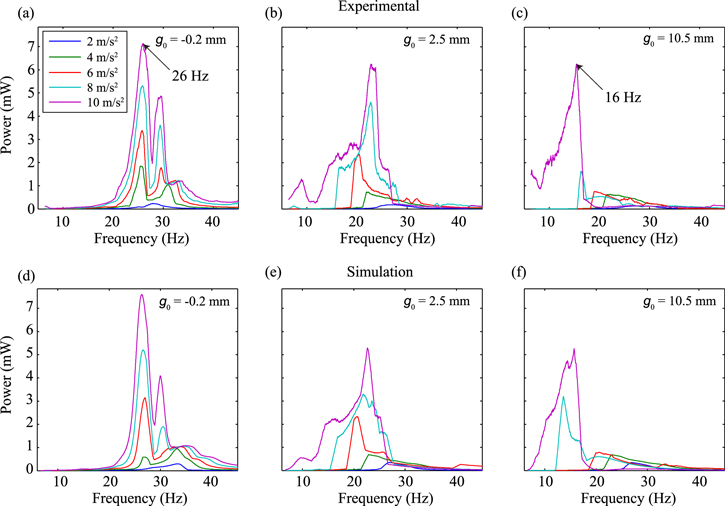
Figure 7. Experimental power (a)–(c) and simulated power (d)–(f) as a function of frequency (forward-sweeps)—Acc = 2–10 m s−2, g0 = −0.2, 2.5, 10.5 mm.
Download figure:
Standard image High-resolution imageTable 1. Model parameters used in forward-frequency sweeps.
| Parameter | Value | Unit |
|---|---|---|
| m1 | 16.725 | g |
| m2 | 5.433 | g |
| k1 | 910 | N m−1 |
| k2 | 570 | N m−1 |
| k3 | 910 | N m−1 |
| dmag | 8 | mm |
| Bres | 1.35 | T |
| ri | 6.6 | mm |
| ro | 8.5 | mm |
| ctax | 5.333 | mm |
| N | 2763 | — |
| Rc | 307.2 | Ω |

|
0.02 | — |

|
0.01 | — |

|
7.73 | s−1 |

|
6.79 | s−1 |
The results shown in figure 7 demonstrate the change in response with changing acceleration level and gap length. It is evident that the model captures both the dynamic and electrical behaviour of the harvester, with the changing shape of the frequency response curve with g0 evident in both the experimental and simulation sweeps. For the Acc = 10 m s−2 curves, the frequency at which the peak power occurs is predicted to within 1.3 Hz in each case. The predicted amplitude of the peak power varies more significantly than the predicted frequency, with the largest variation being 27.8%, while the predicted peak power for the remaining g0 values are all within 16%. The reason for the large deviation between the experimental and simulation results for certain conditions (e.g., g0 = 10.5 mm and Acc = 8 m s−2) is that, in this parameter range, the response amplitude is dictated by whether or not the masses achieve a high energy state of motion. The threshold above which this state occurs is extremely sensitive to the model parameters, such as the damping. Therefore, a slight inaccuracy in the model parameters can have a large effect on the predicted output.
- At 2 m s−2, the acceleration is not high enough to induce large oscillations, irrespective of g0. As a result, the masses remain in contact with the springs and the system behaves similarly to a linear harvester. As the acceleration is increased, the masses leave the springs, impacting one another, resulting in velocity amplification of the magnet stack, m2—provided m1 is on an upward trajectory (). The harvester's behaviour becomes increasingly nonlinear with increasing acceleration, with both the amplitude and bandwidth of the response increasing.
- As g0 is increased, the optimal frequency shifts downwards due to the decreasing effective stiffness—a result of the masses spending a portion of each cycle out of contact with the springs. The higher g0, the greater the portion; thus, the greater the reduction in optimal frequency. A shift in the optimal frequency from 26 to 16 Hz—a reduction of 38.5%—is evident in the experimental frequency sweeps at Acc = 10 m s−2, moving from g0 = −0.2 to 10.5 mm, suggesting that g0 could be implemented as a tuning parameter.
- As g0 is increased, the acceleration level required to induce large oscillations also increases. For g0 = 10.5 mm, an acceleration level of 10 m s−2 is required to achieve a high RMS velocity response. At acceleration levels lower than this, the magnet stack does not engage the stopper spring and high velocities are not achieved. This requirement of a large input acceleration to achieve a significant response affects the applicability of VAEGs for applications featuring low accelerations.

5.2. Performance metrics
The performance of the 2-DoF VAEG is described using the metrics normalised power density (NPD) [8] and volume figure of merit (FoMV) [24]. The highest NPD and FoMV from the results in figure 7, and the corresponding geometric and excitation conditions, are listed in table 2. The VAEG volume prescribes the virtual cylinder surrounding the device, with diameter equal to the outer coil diameter, and height equal to the distance from the top of the base to the bottom of the cap.
Table 2. Highest NPD and FoMV for dmag = 8 mm, air-gap = 2.6 mm.
| g0 | Vol | Acc | f | P | NPD | FoMV |
|---|---|---|---|---|---|---|
| mm | cm3 | m s−2 | Hz | mW | kg s m−3 | % |
| −0.2 | 17.42 | 4 | 25.5 | 1.85 | 6.64 | 0.53 |
| 10.5 | 20.08 | 10 | 15.4 | 6.26 | 3.12 | 0.98 |
Simulation forward-frequency sweeps were completed for the dmag = 12 mm harvester with an air-gap that would apply if the coil was wound directly around the Teflon tube, rather than around the adjustable coil holder. The model parameters used were the acceleration, gap length and coil position resulting in maximum NPD and maximum FoMV in table 2. The simulation results predict that by winding the coil directly around the tube, the highest FoMV and NPD values can be increased by factors of 2.89 and 4.42, respectively, with the predicted values listed in table 3.
Table 3. Highest NPD and FoMV for dmag = 12 mm predicted from simulation sweeps—coil wound directly around the Teflon tube, air-gap = 1.8 mm.
| g0 | Vol | Acc | f | P | NPD | FoMV |
|---|---|---|---|---|---|---|
| mm | cm3 | m s−2 | Hz | mW | kg s m−3 | % |
| −0.2 | 28.2 | 6 | 29.6 | 29.98 | 29.54 | 2.59 |
| 10.5 | 31.1 | 10 | 16.4 | 34.51 | 11.10 | 2.83 |
Considering the frequency range in which the harvester operates (<30 Hz), the predicted performance values presented are reasonably high (see table 4 to compare the presented performance metrics with those of electromagnetic VEHs from the literature). The results demonstrate that velocity amplification is an effective method of achieving high power output at low frequencies, provided the acceleration is sufficiently high to achieve large amplitude oscillations.
Table 4. Summary of electromagnetic VEHs reported in the literature.
| Vol | Acc | f | P | NPD | FoMv | |||
|---|---|---|---|---|---|---|---|---|
| Author | Year | References | (cm3) | (m s−2) | (Hz) | (μW) | (kg s m−3) | (%) |
| Spreeman et al | 2006 | [35] | 1.50 | 28.0 | 80.0 | 3000 | 2.55 | 1.028 |
| Beeby et al | 2007 | [8] | 0.15 | 0.6 | 52.0 | 46 | 883.97 | 24.838 |
| Saha et al | 2008 | [36] | 12.70 | 0.4 | 8.0 | 14.6 | 7.93 | 0.213 |
| Ferro Solutions | 2009 | [37] | 170.00 | 1.0 | 60.0 | 5200 | 30.59 | 0.121 |
| Xing et al | 2009 | [38] | 69.00 | 5.6 | 54.0 | 5000 | 2.31 | 0.077 |
| Hatipoglu et al | 2010 | [39] | 4.10 | 1.0 | 24.4 | 144 | 35.12 | 1.185 |
| Park et al | 2010 | [40] | 0.60 | 7.9 | 54.0 | 115 | 3.07 | 0.702 |
| Cepnik et al | 2011 | [41] | 10.00 | 9.9 | 50.0 | 20600 | 21.15 | 2.554 |
| Cepnik et al | 2011 | [42] | 1.20 | 1.0 | 143.0 | 12 | 10.00 | 0.087 |
| Elvin et al | 2011 | [43] | 2.30 | 1.0 | 112.3 | 8 | 3.48 | 0.031 |
| Perpetuum | 2013 | [44] | 135.00 | 2.0 | 100.0 | 20000 | 37.04 | 0.190 |
| Ashraf et al | 2013 | [45] | 27.38 | 9.8 | 18.0 | 9360 | 3.56 | 0.847 |
| Munaz et al | 2013 | [46] | 9.05 | 4.9 | 6.0 | 4840 | 21.92 | 11.412 |
| Nico et al | 2016 | [19] | 8.12 | 3.9 | 11.5 | 2060 | 16.51 | 2.600 |
6. Scaling
The influence of scaling on VAEGs, in comparison to linear harvesters, is discussed in this section. In section 6.1, an overview of the state-of-the-art in the scaling of linear electromagnetic energy harvesters is presented. As this is in relation to linear systems, the scaling of the mechanical and electrical systems can easily be considered by analysis of the complete system. Section 6.2 addresses the influence of scaling on a 2-DoF VAEG. The device characterised in section 5 was fabricated at three scales, with the device undergoing homothetic scaling, i.e. it was scaled equally in all directions. The three device scales ranged in volume from ∼4.5 to 60 cm3. These systems were nonlinear, which increases the complexity of the scaling analysis, compared to linear systems. Consequently, to investigate the influence of scaling on the VAEGs, the electrical and mechanical systems are considered separately.
6.1. Linear scaling theory
Summarised in this section is the scaling theory of linear inertial energy harvesters, as presented in the literature. The critical parameters are introduced and their scaling relationships are discussed in section 6.1.1. In section 6.1.2, an analytical approach to explore different mechanical damping scaling relationships is presented, with two scaling relationships considered.
6.1.1. Scaling of a linear electromagnetic harvester
The length scale, s, of a harvester is defined as the cubed root of the device volume (s = Volume1/3). It was shown by [24] that the maximum average power dissipated by a linear energy harvester per cycle at resonance is  . The displacement limit of the mass Zlim scales with the length scale (Zlim ∝ s), while the mass scales with the volume (m ∝ s3). The excitation amplitude Y and resonant frequency ωn are independent of scale; therefore, it is stated that the maximum power scales as Pmax ∝ s4. However, the mechanical damping, cm, is not accounted for in the analysis of [24].
It was demonstrated by [22] that the scaling rate of the actual displacement amplitude, Zmax, is affected by cm, which also affects the electrical damping, ce, required to maximise the power delivered to the load (electrical domain analogue matching (EDAM) condition, [47]). Consequently, although Zlim—the maximum possible displacement of the mass within a device volume—scales with s, the assumption that Zmax ∝ s may not be valid. An expression of the maximum power delivered to the load at the optimal load resistance was derived by [47]:
Assuming that all of the harvester components are scaled uniformly with s, the scaling relationships of the parameters in (12) and other relevant parameters are as listed in table 5—a parameter which is ∝s0 is independent of scale. Clearly, in order to determine the load power scaling rate from (12), the scaling relationship of the mechanical damping must be known. This is discussed in the following subsection.
Table 5. Scaling relationships of the parameters in a linear electromagnetic harvester.
| Parameter | Symbol | Relationship |
|---|---|---|
| mass | m | ∝s3 |
| Base acceleration | Acc | ∝s0 |
| Coil volume | Vcoil | ∝s3 |
| Coil wire diameter | dw | ∝s |
| Coil wire area |

|
∝s2 |
| Coil wire length |

|
∝s |
| Fill factor | ff | ∝s0 |
| Coil resistance |

|
∝s−1 |
| Resistivity of copper | ρcop | ∝s0 |
| Coupling coefficient |

|
∝s |
| Radial flux density | Br | ∝s0 [23, 48] |
6.1.2. Mechanical damping scaling
In the following analysis, the influence of the mechanical damping coefficient, cm, on scaling is considered. The scaling of cm is more difficult to define than the previously discussed parameters as it comprises a number of damping mechanisms including thermoelastic damping, friction, squeeze-film damping, and air resistance. The dominant damping mechanism is dependent on the device design and fabrication. It is stated by [22] that viscid damping is usually dominant, and scales as cm ∝ s. This scaling relationship is also taken by [25].
In this analysis, two mechanical damping scaling rates are considered— and cm ∝ s3. The former, cm ∝ s, is the scaling relationship which is typically employed. The latter mechanical damping scaling condition, cm ∝ s3, is discussed here as it is employed in the investigation into energy conversion in the transducer of a VAEG in section 6.2.1, and it is of interest to investigate this effect on linear systems in order to allow direct comparison to the VAEG systems.
 : Inserting
  [22] into (12) yields the scaling relationship for linear oscillatory energy harvesters for the given mechanical damping scaling relationship:
As the denominator of (13) contains a sum, two asymptotic scaling relationships can be determined:


These scaling relationships were described by [22] based on analysis of the equations derived by [47].
From (13), where the electrical damping dominates ( ) the scaling relationship approaches PL ∝ s5. If, however, the mechanical damping dominates (
 ) the scaling relationship approaches PL ∝ s7. Examination of the scaling relationships of these terms—
 and cm ∝s—suggests that at larger scales electrical damping will dominate, while at smaller scales mechanical damping will dominate.
The amplitude of the mass displacement scales at a minimum rate of Zmax ∝ s2, i.e. the displacement of the mass decreases at a greater rate than the displacement limit, Zlim. This is determined by inputting the scaling relationships described above into the equation for maximum displacement amplitude,  . Clearly, assuming cm ∝ s, scaling has a highly negative effect on the power density of a linear VEH, with a minimum load power scaling rate of PL ∝ s5.
 : This is the ideal case where the mechanical damping scales directly with the volume, and so, the damping is independent of scale. This scaling relationship is unlikely to occur in reality, as the difficulty of fabricating devices with moving components increases as scale is reduced, while aspects of the device such as surface finish become more significant. However, it is informative to understand the influence of this damping scaling relationship, as it allows the scaling behaviour of the system and its parameters to be investigated independent of damping:
- In this instance, the mechanical damping and, consequently, the electrical and total damping scales with the volume ()—EDAM load matching condition [47].
- The total damping ratio ζT is, therefore, independent of scale (, where m ∝ s3 and ωn ∝ s0),
- Zmax remains constant () and
- PL ∝ s3 (12).

Zmax does not scale under this mechanical damping scaling condition as the total damping force acting on the mass scales in proportion to the volume, resulting in the motion of the mass (its velocity–frequency response) remaining constant with scale (this is shown explicitly in figure 11(a) for a 2-DoF VAEG). This is only possible if the displacement limits do not scale with the other harvester dimensions. If the spring deflection limit, Zlim, is less than Zmax, obviously, the mass would not be able to oscillate to its maximum displacement.
6.2. Scaling of a 2-DoF VAEG
As the systems described in section 6.1 were linear, the influence of scale on the individual parameters could be determined readily through analysis of the equations of the coupled system. In the scaling analysis of a 2-DoF VAEG, described in this section, the influence of scale on the system response cannot be determined readily from the system equations, as the relationships between the individual parameters and the harvester response vary nonlinearly. For example, the displacement response of the individual masses in the 2-DoF VAEG change nonlinearly with the input excitation level, which has a direct effect on the harvested power. Linear systems do not contain parameters of such complexity. Clearly, determining the causes of variations in VAEG response at different scales while considering the entire system would be difficult. Consequently, to determine the influence of the individual parameters on the response as scale is reduced, particularly the gap length and excitation amplitude, the electrical and mechanical responses are decoupled, in as much as this is possible, and examined separately at different scales. This reduces the number of parameters which may be affecting the response in each case, allowing the influence of the individual parameters to be assessed more directly.
To clarify the function of the nonlinear scaling method developed in this section: for a linear system, the nonlinear scaling method predicts the same scaling behaviour as the linear scaling method. However, the linear scaling method cannot be applied to nonlinear systems due to the dependency of certain system parameters on input conditions; therefore, it was necessary to develop the nonlinear scaling method.
Section 6.2.1 explores the influence of scaling on energy conversion in the transducer of a 2-DoF VAEG by isolating the electrical system from the mechanical domain. An analysis of the influence of the mechanical damping scaling rate on the velocity–frequency response of a 2-DoF VAEG is presented in section 6.2.2.
6.2.1. Influence of scaling on energy conversion in a VAEG
Implementation: In the analysis of the influence of scaling on energy conversion in the transducer of a VAEG, presented in this subsection, a number of deviations from the linear scaling theory of [22] are employed. The purpose of these deviations is to achieve, as closely as possible, conditions where the mechanical damping scales directly with the volume (cm ∝ s3); hence, maintaining the velocity–frequency response across scales. This allows the effect of scaling on energy conversion in the transducer to be considered separately from the mechanical system, i.e. any difference in energy converted in the transducer is a result of the electrical, rather than the mechanical system. The deviations employed in the analysis of the influence of scaling on the electrical system of a 2-DoF VAEG are discussed below.
- The mechanical damping coefficient was assumed to scale with volume (cm ∝ s3) in the simulations, rather than the dimension (cm ∝ s), as in [22].
- As described in section 6.1.2, under the damping scaling rate , the displacement amplitude does not scale. To accommodate this, the spring height was not reduced with scale (hspring ∝ s0) in both the experimental and simulated scaling analysis. This avoided the possibility of the displacement exceeding the maximum spring compression. Additional height contributed by the springs was not considered in the volume and corresponding length scale. The volume used to define the length scale (s = Volume1/3) was, therefore, the product of the area within the outermost coil, and the summed height of the copper mass, magnet stack and gap. A schematic showing the influence of scaling on the geometry of the 2-DoF VAEG in the current experimental and simulation scaling analysis is illustrated in figure 8, with the area contributing to volume highlighted. Evidently, the copper mass and transducer dimensions scale with s, while the spring height does not scale. Initial gap, g0, does not scale either—the reason for this is described in the following point.
- The geometric feature of a VAEG which differs most significantly to a linear energy harvester is the presence of an initial gap, g0, between the masses and springs. As g0 is a component of the displacement range, it does not scale; this means that the change in dynamics with g0 is independent of scale and g0 must remain constant to maintain the velocity–frequency response with scale. This is a consequence of the effective stiffness of the harvester being dependent on the portion of the cycle the masses spend attached/detached from the springs during operation. For the effective stiffness to be maintained and, consequently, the velocity–frequency response to be the same across scales, the portion of each cycle the masses spend in contact with the springs must remain constant. Consequently, in the analysis presented, g0 remains constant with scale. As a result of this, the rate of change of volume with magnet coil dimension decreases as g0 increases, i.e. the larger g0, the smaller the influence of scaling on its volume. The scaling relationship is described for a range of g0 values.
- Uniform scaling of the dimensions of a uni-axially loaded spring—which can be of cantilever, helical, or planar form—results in the spring stiffness scaling as k ∝ s [49]. Consequently, the natural frequency is inversely proportional to length scale (wn ∝ s−1). In this analysis, the spring stiffness, k, was scaled as k ∝ s3, such that the natural frequency of an equivalent linear system would remain constant with scale ().


As a result of the scaling conditions described above, the system dynamics—amplitude and frequency of velocity and displacement responses—were not affected by scale in the scaling analysis of VAEGs presented. The electrical system was, thus, partly isolated from the mechanical system. Any deviations from linear scaling theory were then a result of the effect of scaling on energy conversion in the transducer. The difference in the effect of scaling on a linear system and a VAEG can, therefore, be determined solely in terms of the transduction properties. This is the defining feature of the scaling analysis presented in this section, allowing the mechanical and electrical systems to be considered separately across scales.
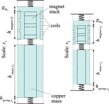
Figure 8. Schematic showing the cross section of a 2-DoF VAEG at scales s1 and s2. Dimensional scaling relationships:  ,
,  ,
,  .
.
Download figure:
Standard image High-resolution imageAs previously stated, if the transducer is scaled uniformly, the transducer properties scale as follows: dw ∝ s, lw ∝ s, Aw ∝ s2, RC ∝ s−1 and K ∝ s. In the scaling analysis presented in this section, the coil wire diameter was kept constant (dw ∝ s0) so that the coil fill factor would be the same for each scale; whereas, if the coil wire diameter was scaled, the fill factor would likely have changed and this would have affected the uniform scaling of the VAEGs. Applying the same analysis as above to the systems with constant coil wire diameter gives: lw ∝ s3, Aw ∝ s0, RC ∝ s3 and K ∝ s3. Inserting these scaling relationships into (12) yields the same scaling relationships described for dw ∝ s, i.e. the load power scales at the same rate for both dw ∝ s and dw ∝ s0 (PL ∝ s3). This is because the scaling rate of the RC/K2 term in (12) remains the same for both cases, i.e.  . A constant coil wire diameter of dw = 100 μm was used in this analysis.
The scaling relationships employed in the scaling analysis of a 2-DoF VAEG are summarised in table 6. Parameters described as uniform scaling are those which conform to homothetic scaling, or the scaling relationships employed by [22]. The non-uniform scaling parameters are those which do not conform to homothetic scaling, while the resultant parameters are those whose scaling relationships are a consequence of the non-uniform scaling.
Table 6. Scaling relationships employed in the simulation scaling analysis of a 2-DoF VAEG.
| Parameter | Scaling relationship | |
|---|---|---|
| Uniform scaling | m | ∝s3 |
| Vcoil | ∝s3 | |
| Br | ∝s0 | |
| Non-uniform scaling | cm | ∝s3 |
| dw | ∝s0 | |
| g0 | ∝s0 | |
| k | ∝s3 | |
| Resultant | Aw | ∝s0 |
| RC | ∝s3 | |
| lw | ∝s3 | |
| ce | ∝s3 | |
| K | ∝s3 | |
| wn | ∝s0 | |
Examining (12), with cm ∝ s3, the only parameter which could cause a deviation from PL ∝ s3—the linear scaling relationship—is K, as the remaining parameters are rigidly defined. A variable K becomes Keff, the effective electromagnetic coupling coefficient, which is the RMS of K over a period of excitation:
Although the peak K is proportional to the length scale cubed, Keff can scale at a greater rate. The peak K occurs when the coil and magnet stack are located at the optimal relative position—which is determined by the geometry of the transducer. For small displacement ranges, Keff remains close to this peak value. In VAEGs, the displacement range varies with g0; the larger g0, the greater the displacement range (provided the excitation conditions result in large amplitude oscillations). Large displacements result in values of Keff which are considerably lower than the peak value. The relative position of the magnet and coil which results in maximum average power generation, for a set of excitation conditions and a given g0, differs from the optimal relative magnet coil position under very low displacements. In this case, the optimal magnet coil position is the one that results in the highest RMS load voltage, which is a function of K and relative velocity.
In the simulations,  and the velocity–frequency response remained constant with scale. In the experimental data (figure 10), this was not the case; cm scaled at a lower rate, resulting in the mechanical damping effect increasing as scale was reduced. Consequently, the experimental velocity response did not remain constant with reduced scale; its amplitude reduced. To allow the experimental and simulation results to be compared across scales, rather than using the load power, the effective coupling coefficient was employed. This was appropriate as Keff is normalised by velocity, which mitigates the issue of the experimental velocity–frequency response amplitude changing with scale.
The voltage induced in the electrical circuit was derived using Kirchhoff's voltage law in (8). As the harvester is designed to operate at low frequencies (<30 Hz), the effect of the coil inductance was small [50] and, hence, was neglected here—the inductor impedance was ZL = 56 Ω at 30 Hz, compared to a coil resistance of RC = 938.9 Ω. Rearranging (8) allows an expression for the load voltage to be found:
where v is the relative velocity between the magnet and coil. The effective coupling coefficient Keff is calculated from both simulation and experimental data by rearranging (16):
In this case VL is the RMS load voltage, while v is the RMS velocity.
The experimental Keff is calculated from the peak RMS load voltage and the corresponding RMS velocity in the experimental frequency sweeps. Although the RMS relative and absolute velocities vary significantly at frequency ranges above and below the peak frequency, the deviation between them is small at the peak frequency. This is illustrated in figure 9 for simulation frequency sweeps at a range of g0 values, and the findings are valid for all scales—under the mechanical damping conditions employed. As the LDV measures the absolute velocity of the mass, and due to the small difference in absolute and relative RMS velocities at the peak response, the RMS absolute velocity is used in the calculation of the experimental Keff.
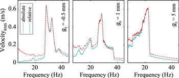
Figure 9. Absolute (- - - -) and relative (—–) RMS velocity of m2 for simulation forward-frequency sweeps at a range of gaps—Acc = 10 m s−2, R = 3, s ≈ 19 mm.
Download figure:
Standard image High-resolution imageResults: The simulation and experimental Keff are plotted as functions of the length scale in figure 10 for acceleration levels of Acc = 10 and 6 m s−2, for gap lengths ranging from g0 = −0.2 to 10.5 mm. The experimental data is plotted for the three magnet diameters, dmag = 6, 8, and 12 mm, while the simulation data is presented for magnet diameters in the range dmag = 4.3–15.6 mm (range selected to extend beyond experimental range to higher and lower scales). The simulation data was taken at a single frequency which varied for each g0 and acceleration. The selected frequency remained constant with scale, however. This single frequency was selected based on the response showing a high amplitude over the entire range of scales at this frequency.
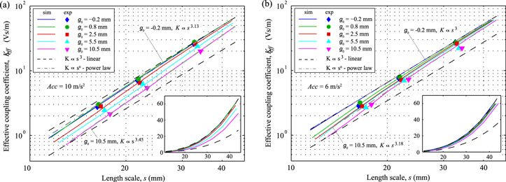
Figure 10. Experimental and simulation effective coupling coefficient, Keff, as a function of length scale, for a range of g0; (a) Acc = 10 m s−2 and (b) Acc = 6 m s−2—main graphs plotted on logarithmic scales, embedded graph plotted on linear scales.
Download figure:
Standard image High-resolution imageThe results of the scaling analysis of a 2-DoF VAEG are discussed below.
- The linear scaling relationship, K ∝ s3, is plotted as two dashed lines from the maximum and minimum Keff values, respectively (figure 10). These lines are included to compare how the scaling behaviour of the 2-DoF VAEG deviates from the linear scaling relationship.
- Evidently, Keff scales at a greater rate than the linear relationship. This is due to the aforementioned reduction in Keff with increased displacement range, which is a consequence of the relative motion of the magnet stack and coils being in sub-optimal locations for portions of each cycle.
- At higher values of g0, the scaling rate of Keff is increased further. This is a result of g0 remaining constant with length scale, which causes the volume to decrease at a slower rate than s3. The increased scaling rate of Keff is seen in the shift in experimental data points to higher length scales with increasing g0, and in the divergence of the simulation results from each other and the linear scaling relationships as length scale is decreased.
- Furthermore, as the magnet stack and coil dimensions are reduced, Keff is effectual over a smaller range, which becomes an ever smaller portion of the displacement range.
- Power law relationships are fitted to the simulation results for the highest and lowest gap lengths.
- In the simulation results, at the lowest acceleration level (Acc = 6 m s−2) and the lowest gap (g0 = −0.2 mm), the scaling rate is effectively the same as for a linear system (K ∝ s3). This is because, under these excitation and geometric conditions, the harvester effectively behaves as a linear system, i.e. the masses are always in contact with a spring.
- As g0 and the acceleration level are increased, the displacement range rises and the system no longer behaves linearly. The scaling rate increases as a result of this larger displacement range. At the highest acceleration level (Acc = 10 m s−2) and the highest gap size ( mm), the highest scaling rate of K ∝ s3.45 is seen.

The scaling analysis described here relates to VAEGs; however, the results are also relevant for other electromagnetic energy harvesters which operate at low frequencies featuring large displacement amplitudes [13, 51]. In these systems, Keff will be lower than the peak K, and will scale at a greater rate than a system featuring lower displacement amplitudes. This indicates that inertial generators operating at low frequencies will scale poorly, compared to devices operating at higher frequencies.
6.2.2. Influence of mechanical damping scaling in a VAEG
The influence of the mechanical damping scaling rate on the velocity–frequency response of a 2-DoF VAEG is investigated in this subsection. This analysis is of interest as it explores the limits of damping on the dynamic response of a VAEG. The focus of the scaling analysis presented thus far has been on the influence of geometry and acceleration level on the scaling of the electrical system of a VAEG, relative to that of a linear system. Simulation only is employed in this analysis; the experimental mechanical damping scaling rate is not considered, as the mechanical damping parameters are highly dependent on the fabrication quality. A sample of three fabricated devices is, consequently, not significant enough to draw conclusions of significance from. This section compares the velocity–frequency response of 2-DoF VAEGs at four length scales for three mechanical damping scaling rates, through simulation.
The dominant component of mechanical damping in a VEH is highly dependent on the device design. In the VAEG demonstrated herein, the most significant components of the mechanical damping were thermoelastic damping in the springs, and friction between the masses and Teflon tube.
Simulation velocity–frequency responses for a range of mechanical damping scaling rates and length scales are presented in figure 11. This test series was completed to show the influence of the mechanical damping scaling rate on the frequency response of a 2-DoF VAEG. Scaling rates of cm ∝ s3, cm ∝ s2, and cm ∝ s are presented for four length scales. The reasons these scaling rates were selected are as follows: cm ∝ s3—the ideal scenario, with the velocity–frequency response remaining constant as scale is reduced; cm ∝ s—the scaling rate stated by [22]; and cm ∝ s2—shows the transition between the two previously described scaling rates. The length scales presented are lower than those in figure 10, as there is no coil present—the dynamics only are under investigation—which decreases the device volume.
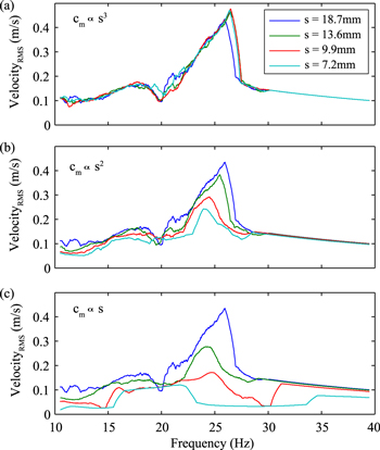
Figure 11. Simulation frequency forward-sweeps showing RMS velocity of magnet stack for a range of length scales; (a) cm ∝ s3, (b) cm ∝ s2, and (c) cm ∝ s—Acc = 10 m s−2, g0 = 2.2 mm.
Download figure:
Standard image High-resolution imageFor  , the system velocity–frequency response does not change with scale (figure 11(a))—as discussed in section 6.2.1. Lowering the scaling rate results in the RMS velocity significantly decreasing with scale. The mechanical damping dominates, such that the masses no longer achieve high velocity impacts that result in velocity amplification. This is particularly evident in figure 11(c), where the peak demonstrated at higher length scales is no longer present at s = 7.2 mm. Comparing the highest and lowest length scales presented for cm ∝ s, the peak RMS velocity of the magnet stack goes from 4.36 to 1.21 m s−1, which is a reduction of 72.4%. This has a highly negative effect on the potential energy which can be harvested from a VAEG, particularly approaching MEMS scale.
Considering, finally, the scaling of the load power in a 2-DoF VAEG, assuming cm ∝ s. Incorporating a transducer in the model used in figure 11 allowed the power generated at each scale to be simulated. Going from a length scale of s = 18.7 to 8.4 mm (the increase in volume with the addition of the coil is neglected to keep the length scales consistent with figure 11), the simulated peak power generated drops from PL = 12.48 to 0.152 mW. This corresponds to a scaling rate of PL ∝ s5.51, which is in the range specified by [22] (14a). Decreasing the scale further, this power scaling relationship continues to increase, as the influence of the mechanical damping increases relative to the electrical damping, becoming the dominant damping mechanism. This is further compounded by the volume decreasing at a lower rate than the transducer dimensions, due to g0 remaining constant with scale.
7. Conclusion
A 2-DoF VAEG with a mass ratio of R = 3 was fabricated at three scales. A nonlinear scaling method was developed to allow the scaling behaviour of the nonlinear 2-DoF VAEGs to be determined. The main features of this method were:
- The complexity of the nonlinear system was reduced by partly isolating the electrical system from the mechanical system, allowing the influence of scaling on the energy conversion in the transducer to be determined.
- This was done by maintaining the velocity–frequency response of the mechanical system across scales. To achieve this, the mechanical damping coefficient and the spring stiffness were scaled with volume, while the displacement range was not scaled.
- The effective electromagnetic coupling coefficient was employed to analyse the scaling behaviour, as it is normalised by velocity. This mitigated the effect of changing velocity with scale on the output.
One of the three fabricated harvesters was characterised using frequency sweeps for a range of cap heights and acceleration levels through simulation and experimentation.
- A shift in optimal frequency to lower frequencies with increasing gap length, g0, was demonstrated. This shift was a result of reducing effective stiffness, with the masses spending a smaller portion of each cycle in contact with the springs.
- It was observed that the input acceleration level required to generate large amplitude oscillations at the optimal frequency increased with g0.
The three harvesters were tested to determine the influence of scale on a VAEG, relative to a linear energy harvester.
- It was determined that if the frequency response of a VAEG is to be maintained with scale, the initial gap, g0, must be kept constant, i.e. g0 does not scale. A consequence of this is that the total device volume scales at a slower rate than the transducer dimensions, which reduces the power density as scale is reduced.
- The scaling rate of the effective electromagnetic coupling coefficient, Keff, is greater than that of a linear system (Keff ∝ s3), with rates of predicted. This is due to the larger displacement range, with the magnet and coil spending large portions of each cycle in sub-optimal relative positions. The scaling rate of Keff in a VAEG increases with increasing g0 and excitation acceleration as the effect of the sub-optimal coil-magnet position is compounded.
- The scaling rate of Keff increases with displacement amplitude. This means that electromagnetic VEHs operating at low frequencies will scale poorly compared to systems operating at higher frequencies.
- Considering the scaling of the mechanical system, if the mechanical damping scales at cm ∝ s, the effects on the RMS velocity of the transducer mass are severe, with a reduction of 72.4% in peak RMS velocity predicted in reducing from a length scale of s = 18.7–7.2 mm.
- Recombining the mechanical and electrical systems for the same mechanical damping parameters, the load power was predicted to scale as PL ∝ s5.51. Clearly, this has negative implications for the feasibility of a 2-DoF VAEG at micro-scales.

Acknowledgments
The authors acknowledge the financial support of Science Foundation Ireland under Grant No. 10/CE/I1853 and the Irish Research Council (IRC) for funding under their Enterprise Partnership Scheme (EPS). Bell Labs Ireland would also like to thank the Industrial Development Agency (IDA) Ireland for their continued support.