

Abstract
Optimal operation, reduced energy consumption, longer service availability, and high safety level are the major concerns in today's railway transport systems. Smart monitoring systems should address these issues without interrupting railway operability. Many successful works have been carried out to provide railway monitoring functions using fiber Bragg grating (FBG) sensors on rail. Most of them are based on strain measurement due to the train passage. This paper presents a highly sensitive means for railway monitoring based on vibration measurement. FBG accelerometers placed on sleeper have been employed as sensor heads, which significantly facilitated the field sensor installation work compared to the positioning on the foot of the rail. An optimized signal demodulation algorithm has been effectively used to extract from the accelerometer traces both the axle number and the average speed information. Excellent capability of the developed system to obtain both parameters has been demonstrated by the way of field trials carried out on a Belgian railway line, during its normal operation. Easy installation, multi-function diagnosis, good data integrity, and compatibility with fiber optic sensors make the proposed sensor a good candidate for railway monitoring applications.
Export citation and abstract BibTeX RIS
1. Introduction
Today's railway operating systems are characterized by trains operating under high loads at very high speeds, widespread use of freight trains, and substantial increase in the overall traffic [1]. All of these factors make any failure more disastrous than before, creating a significant pressure on the maintaining and inspection methods. This concern can only be addressed by using effective control and monitoring techniques of the physical infrastructure. Both wayside and on board measurement approaches have been extensively studied in the literature providing condition monitoring data for the diagnosis as well as prediction of failures [2, 3].
Most of current trackside signaling systems do not have the speed of the trains as an input data. The train movement information is limited to the succession of track circuits for which axle counting is an elementary security measure. In these systems, as a train passes, the number of axles is counted. Two of such subsequent counting units determine whether the train is on a particular section or not [4–6]. The conventional technology to realize axle counting is based on magnetic sensors. While this sensing technology is, well-known and consolidated, it has got a major drawback: adverse effect of electromagnetic interferences (EMI). This problem has been aggravated with electrification (high-voltage overhead lines), power electronics (traction drive systems), and magnetic breaks (large metal pieces mounted on the bogie of the vehicle) leading to false alarms, unstable and faulty operation of trains [4–6].
The train speed is measured on-board for operational and safety purposes but it is not reported to the trackside system in a majority of situations. Gaining access to the train speed data directly at trackside enables to optimize the performance of crucial signaling functions. For instance, the traffic management and regulation system can provide more accurate services. Moreover, the behavior of level crossings can be optimized. The warning time (between announcing the approach of the train to the road users and the closing the barriers) can become a function of the train speed rather than a constant value calculated on the basis of the maximum train speed.
In this context, fiber optic sensors, particularly fiber Bragg gratings (FBG) have been attracting a growing interest in the research community [4]. The tendency toward accepting FBGs as an alternative solution in railway monitoring is largely due to many advantages of these mass producible intrinsic sensing devices, such as inherent wavelength-encoded demodulation feature, resistance to EMI, great configurability with multiplexing capability (several tens of cascaded sensors at different wavelengths within a single optical fiber can be interrogated using only one equipment) and remote operation, passive and lightning/corrosion resistive nature, as well as their small size.
Through real time field trials, usage of FBG sensors has already been demonstrated as a feasible solution in train identification, axle counting, defect determination, flat wheel detection, measurement of lateral displacement, speed and acceleration estimation [5–12]. In almost all of these demonstrations, the FBG sensors were manually placed on particular locations (or orientations) and bonded to the foot of the rail (ideally between a sleeper bay [13]). This is a difficult and time consuming process as it requires a careful surface cleaning (e.g. rust removing and polishing), special kind of glues (e.g. cyanoacrylate, UV-photo-polymerized urethane-acrylate), good mechanical protection (e.g. reinforced tubes, armored cables) and more importantly, service disruption during the sensor installation (i.e. direct and secure access to rails). Therefore, there remains ample room for concurrent minimally-invasive railway monitoring approaches as no commercial product based on optical fiber sensors is currently deployed for safety monitoring. The solutions based on FBGs face with the conservative attitude of railway industry, in replacing the proven conventional equipment by innovative counterparts.
In order to meet these stringent outside field requirements, we implemented in this work, the concept of using FBG-based accelerometers positioned on the sleepers rather than the rail. To achieve this objective, we developed an original signal demodulation method to extract the useful information from somewhat noisy traces (due to the very high sensitivity of the sensor head) recorded by the fiber optic accelerometers.
We successfully demonstrated the feasibility of the proposed system for axle counting and train speed determination, through of field trials that were carried out in the Mons–Liège regional railway line, during its normal operation. The results were compared to data obtained by the previous implementation based on FBG strain sensors [5] and to that of simultaneous video recordings. A very good agreement obtained from the comparison proves the efficiency of the proposed demodulation method.
In the following, we will first describe the field instrumentation details and the original demodulation technique implemented to deduce the axle counting and speed information. Finally, we will present the results and compare them with the other techniques.
2. Instrumentation
2.1. FBG-based accelerometer
From a general point of view, fiber optic accelerometers based on FBG technology not only benefit from all the advantages of fiber optic sensors but offer also an important instrumentation capability that is not possible using conventional accelerometers: compatibility with FBG-based strain and temperature sensors, thereby enabling the operation of fiber-based sensing networks. In our work, we benefit from this feature by taking the measurements using both FBG strain sensors and FBG-based accelerometers interrogated by the same equipment from a remote location.
As sketched in figure 1(a), a typical FBG accelerometer includes a flexible cantilever with an FBG mounted on it at one end, and a mass at the other end. When a vertical acceleration is applied on the cantilever beam, a varying axial strain is created on the grating (due to the alteration of flexion and compression), which is proportional to the distance from the neutral axis. The induced strain is demodulated by measuring the corresponding Bragg wavelength shift (alternating between positive and negative extremes).
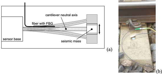
Figure 1. (a) Schematic representation of the FBG accelerometer, (b) photograph of the accelerometer placed on the sleeper.
Download figure:
Standard image High-resolution imageIn our implementation, a commercial accelerometer (OS7100, MicronOptics) with one axis configuration was attached on the sleeper and connected to the sensors network, as shown in figure 1(b). The frequency range of this particular accelerometer was sufficient for both axle counting and speed calculations.
2.2. Railway installation
Fibers connected to the accelerometers, as well as fibers containing the FBG strain sensors were positioned on the Mons-Liège rail tracks (Belgium), nearby the railway station of La Louvière Sud (GPS position of 50.465 643, 4.188 260) in a  i.e. a zone for which the speed of the trains does not exceed 100 km h−1. In general, the train speed at the measurement point is about 30–90 km h−1.
The layout of the whole monitoring system used in our measurements is shown in figure 2. It comprises one FBG accelerometer mounted on the sleeper, various FBG strain sensors placed on the rails, couplers, junction boxes, and the protected feeder cable providing the connection between the sensor network and the interrogator. For a given measurement, the outputs of the FBG strain sensors and the FBG accelerometer are acquired simultaneously on input channels of the interrogator that is located in a remote equipment room. Commercial spectrometer-based interrogators with acquisition rates between 1 and 3 kHz, an absolute wavelength measurement accuracyae of 40 pm and a precision of 1 pm were used in the measurements.
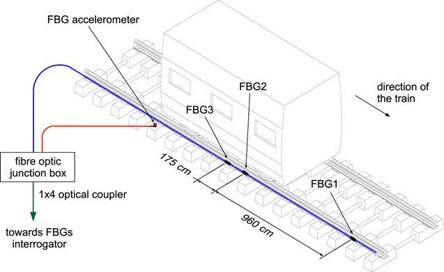
Figure 2. Schematic of the sensors on the Mons-Liège rail track.
Download figure:
Standard image High-resolution image3. Field measurements
Railway monitoring system was tested over a time span of about 6 months, which both allowed relevant statistics on the efficiency and proved the robustness of the overall system. Real-time videos have also been taken from a monitoring camera facility for train identification purpose and reference speed calculation.
The typical traces measured by using the FBG strain sensor and the accelerometer are compared in figure 3. They both correspond to the passage of a 6-car passenger train. The axle positions are clearly visible in the upper trace (FBG strain sensor); whereas some further signal processing is required in the lower case (FBG accelerometer on the sleeper). The noisy nature of the accelerometer output is attributed to the effect of various high frequency components due to the effects of track flexibility and wheel/rail sliding on the vibration signature of the vehicle [14] together with the unwanted residual vibrations of the accelerometer before and after the passage of the wheels. The effect of these vibrations has to be filtered out in our trace analysis, as explained in the following paragraph.
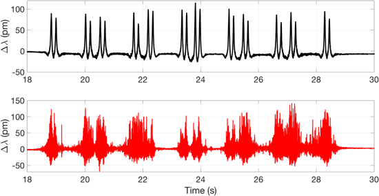
Figure 3. Trace of a 6-car train circulating at 60 km h−1 measured using (a) a FBG strain sensor on the foot of the rail, (b) a FBG accelerometer on the sleeper.
Download figure:
Standard image High-resolution image3.1. Trace analysis
The relationship between the main geometry of the train (i.e. wheel set spacing, bogie spacing and carriage length) and the spectral content of rail vibration has already been demonstrated and successfully validated in a previous work [5]. The periodicity of the axle (La), the bogie (Lb), and the cars (Lc) lead to three different amplitude modulations of the spectrum having corresponding frequency components, fa, fb, and fc. These frequency contents can be calculated as [15, 16]:


in which the vehicle speed is assumed to be constant. In addition to these dominant frequency components, in phase (50–300 Hz) and out of phase (200–600 Hz) vertical vibrations between the rail and the sleepers, together with the pinned-pinned resonances (800–1000 Hz) affect the vertical track dynamics [13]. Moreover, there are residual vibrations recorded by the accelerometer when the wheels are approaching to (and leaving from) the sensor location. These unwanted frequency components have been eliminated by using low-pass filters (LPF) in the proposed trace analysis. Instead of applying a single LPF on the whole trace however, we first divided into segments the raw signal at the accelerometer output. Indeed, the vibration signature (hence the frequency response) corresponding to different parts of the train differ from each other, depending on the train geometry (i.e. the total length, number of cars, and the wheel set positions), the train load and the wheel set conditions. In our analysis, based on the analysis of several raw traces corresponding to different train configurations, this behavior has been validated.
Such a segmentation procedure is demonstrated in figure 4, for a 3-coaches train circulating at about 84 km h−1 (23.33 m s−1). In this example, the raw trace is segmented into 4 parts corresponding to first and last axles, as well as axle pairs of contiguous train coaches. As it can be seen from the figure, the frequency response is different for each segment. Still, for all the segments, the noise components are observed to be significantly stronger in the same frequency range of about 700–800 Hz.
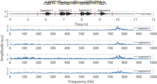
Figure 4. Frequency response of a 3-car train (Desiro AM08 circulating at 84 km h−1) divided into 4 segments corresponding to first and last axles, as well as axle pairs of contiguous train coaches. The train has a wheel set spacing of 2.3 m (La = 2.3 m, fa = 10 Hz).
Download figure:
Standard image High-resolution imageBy taking the frequency value at the center of this dominant noise band (700–800 Hz in this particular example) and applying a multiplication constant, the cut-off frequencies of the individual filters are determined. In this way, for each segment, high frequency vibrations above cut-off frequency are eliminated from the useful low frequency components such as fa (axle periodicity that is related to wheel set spacing, fa = 10 Hz in this example case).
The dominant noise frequencies observed on the raw traces by the on-side measurements (tens of measurements over more than three months on 7 different train types) varied between 150 and 800 Hz. These frequency components are absolutely beyond the frequency range of fa, fb, and fc (e.g. fa would have been equal to 25 Hz even if the train speed had been increased to 200 km h−1. It should also be noted that fa > fb > fc).
Once the segments of the raw trace are low-pass filtered, the envelope detection algorithm is applied on them to determine the axle positions (peaks of the envelope trace). The envelope detection process consists in: first, converting the measured real-valued signal to the corresponding analytic signal (using Hilbert transform), and then, taking the magnitude of this analytic signal. In this process, we implemented the option that applies the spline interpolation over two successive local maxima of the envelope over a given number of samples (i.e. envelope width).
These steps are represented in figure 5 for segment 3 of our example case. The accelerometer output for segment 3 (figure 5(a)) is first low-pass filtered (using Fc−1 = 225 Hz). The vibration signature becomes fine at the output of the filter (figure 5(b)). Envelope of the filtered signal is then found as represented in figure 5(c) (blue line). The width of the envelope detection algorithm is taken as about 1 m, providing the required spatial resolution to resolve wheel positions (distance between axes varies from 2.30 to 2.55 m). Peak search algorithm applied to the envelope trace determines the axle points. In this example segment, the time difference between peaks 2 and 1 is found to be 0.10 s. Using this value and the distance between axles (La = 2.3 m), the instantaneous speed of the train is calculated as 23.00 m s−1 (82.8 km h−1), which is in good agreement with the average speed of the train measured on the reference video. Similar result has been obtained considering the peaks 3 and 4.
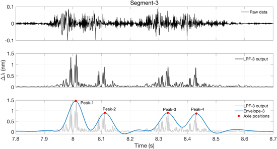
Figure 5. Signal processing steps applied on segment-3 of a 3-car train (Desiro AM08 circulating at 84 km h−1): (a) raw trace, (b) absolute value of the low-pass filter output, (c) envelope applied on the filtered signal, (red points indicate the axle positions determined by peak search algorithm).
Download figure:
Standard image High-resolution imageIn the final stage of the signal processing algorithm, the analyzed segments are merged to re-obtain the global processed signal. Axle positions now being indicated on this signal, the time difference between the last axle and the first axle positions is determined. Knowing the total length of the train, the average speed is then calculated. The flowchart of the signal processing steps applied on the raw trace is summarized in figure 6.
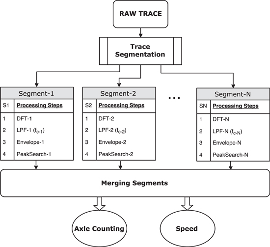
Figure 6. Flowchart of the data processing steps. (DFT: discrete Fourier transform, fc−i: cut-off frequency for the ith segment, LPF: low pass filter). The frequency response of each segment is individually analyzed (by applying FFT algorithm on each segment) to obtain the value of the cut-off frequency to be applied on the filter. Instead of applying one global cut-off frequency, individual cut-off frequencies adapted to the frequency responses of these different parts of the train provide a more effective way to clean vibration noise from the raw signal.
Download figure:
Standard image High-resolution imageFigure 7 represents two traces before and after the proposed data processing steps for our example case (3-car Desiro AM08 train at 84 km h−1). As can be seen in the figure, the axle positions in the raw trace are blurred with the vibration noise components but are clearly resolved after the suppression of this effect with the provided signal processing steps explained above (see figure 6).
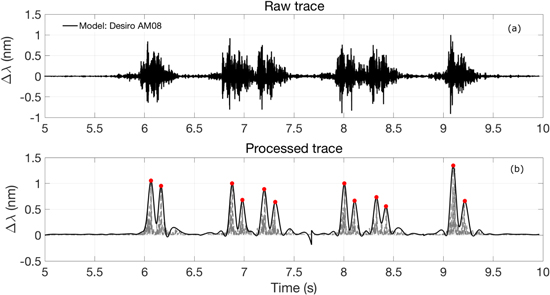
Figure 7. Measured accelerometer response as a function of time induced by a passage of a train (Desiro AM08) with 12 wheels circulating at 84 km h−1 (a) before (b) after the data processing steps (red circles represent the axle points).
Download figure:
Standard image High-resolution image3.2. Results
Thanks to our long-term outdoor installation, numerous field tests were carried out (with intervals of few months) to validate both the hardware of the monitoring system and the related signal demodulation algorithm. Results demonstrate the capability of the proposed system in both counting the number of axles of a given track section (without any miscount), as well as the average train speed estimation. Table 1 summarizes some examples of axle counting and speed measurement results for different train types. Main properties of the tested trains are given in Table 2. Speed values obtained by the proposed system are compared with that coming from FBG strain sensors deployed on the field trial as well as reference videos.
Table 1. Comparison of measured average speed by three methods for ten different trains.
| Train number | Measurement date | Train type | Number of cars | Number of axles (counter result) | Reference speed based on video (km h−1) | Speed based on FBG sensor (km h-1) | Speed based on accelerometer (km h−1) |
|---|---|---|---|---|---|---|---|
| 1 | 21.11.2016 | AM-73 | 2 | 8 | 52.02 | 51.66 | 51.33 |
| 2 | 01.03.2017 | CityRail70 | 2 | 8 | 57.60 | 58.19 | 57.04 |
| 3 | 31.03.2017 | AM-70 | 2 | 8 | 51.41 | 51.40 | 52.65 |
| 4 | 31.03.2017 | AM-78 | 2 | 8 | 36.40 | 38.51 | 39.82 |
| 5 | 31.03.2017 | Desiro AM08 | 3 | 12 | 47.93 | 48.80 | 49.50 |
| 6 | 01.02.2017 | Desiro AM08 | 3 | 12 | 88.62 | NA | 87.80 |
| 7 | 01.03.2017 | AM-96 | 6 | 24 | 65.10 | 63.02 | 64.33 |
| 8 | 31.03.2017 | AM-96 | 6 | 24 | 57.25 | 55.55 | 56.63 |
| 9 | 21.11.2016 | M6 | 7 | 30 | NA | 61.13 | 59.65 |
| 10 | 01.03.2017 | M6 | 7 | 30 | 49.48 | 48.51 | 50.10 |
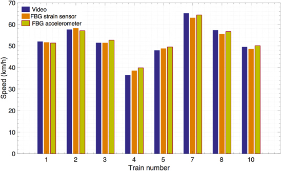
The results provided by the three approaches (video, FBG strain, FBG accelerometer) are presented in figure 8 for the ten different train configurations (train number 6 and 9 are excluded from this figure as one of the reference speed information is missing for these two cases). The error on the reference speed values is determined by the camera resolution (which is 1/30 s). Based on the resolution value and time intervals measured for all the trains, the maximum absolute error was calculated as 1 km h−1.
Figure 8. Train speed estimations compared to FBG strain sensors results and video recordings for ten different trains (train numbers 6 and 9 are excluded from this figure as one of the reference speed information is missing for these two cases).
Download figure:
Standard image High-resolution image
Table 2. Main properties of the tested trains.
| Train type | Number of coaches | Number of axles | Max speed (km h−1) | Distance first-last axle (m) | Total unloaded mass (Tons) |
|---|---|---|---|---|---|
| AM-73 | 2 | 8 | 140 | 38.927 | 107.5 |
| CityRail70 | 2 | 8 | 140 | 39.927 | 104.7 |
| AM-70 | 2 | 8 | 140 | 39.927 | 104.7 |
| AM-78 | 2 | 8 | 140 | 38.927 | 107.5 |
| Desiro AM08 | 3 | 12 | 160 | 70.805 | 141 |
| AM-96 | 6 | 24 | 160 | 151.000 | 314–324 |
| M6 | 7 | 28 | 160 | 180.945 | 348.8 |
4. Conclusions
Some challenging physical conditions characterize railway environments where the remote operation and easy management of sensors are key factors for smart monitoring platforms [17, 18]. The role of enabling technologies (broadband communication, ICT, sensors, etc) to revolutionize the railway industry has been a field of intensive research for more than ten years [19]. Implementations of FBG sensors owe their popularity to their remote sensing capability, where the sensor heads that are not influenced by EMI can be placed along a trackside while the interrogator unit is kept at a safe distance.
In this paper, we presented an efficient method for railway traffic monitoring, which is a very competitive alternative to the use of strain sensors. The critical contribution of this work is the exploitation the FBG-based accelerometer together with the special signal processing demodulation technique that permits us to realize both axle counting and a very good estimate of train speed (±1 km h−1). Their installation can be easily made, without requiring interruption of the railway operability (simpler cabling requirements).
Acknowledgments
This work was financially supported by the INOGRAMS (Innovations for a Global Rail Management System) project (convention 7171) of Wallonia (Belgium) in the frame of the LOGISTICS IN WALLONIA competitiveness cluster. Christophe Caucheteur is an FRS-FNRS Research Associate. The authors thank their industrial partners (Alstom and Infrabel) for fruitful discussions. Kivilcim Yüksel gratefully acknowledges financial support from the TUBITAK (BIDEB-2219-1059B191600612).