
Abstract
Objective. The main objective of this study was to assess the feasibility of lowering the hardware requirements for fast neural electrical impedance tomography (EIT) in order to support the distribution of this technique. Specifically, the feasibility of replacing the commercial modules present in the existing high-end setup with compact and cheap customized circuitry was assessed. Approach. Nerve EIT imaging was performed on rat sciatic nerves with both our standard ScouseTom setup and a customized version in which commercial benchtop current sources were replaced by custom circuitry. Electrophysiological data and images collected in the same experimental conditions with the two setups were compared. Data from the customized setup was subject to a down-sampling analysis to simulate the use of a recording module with lower specifications. Main results. Compound action potentials (573 ± 287 μV and 487 ± 279 μV, p=0.28) and impedance changes (36 ± 14 μV and 31 ± 16 μV, p=0.49) did not differ significantly when measured using commercial high-end current sources or our custom circuitry, respectively. Images reconstructed from both setups showed neglibile (<1voxel, i.e. 40 μm) difference in peak location and a high degree of correlation (R2 = 0.97). When down-sampling from 24 to 16 bits ADC resolution and from 100 to 50 KHz sampling frequency, signal-to-noise ratio showed acceptable decrease (<−20%), and no meaningful image quality loss was detected (peak location difference <1voxel, pixel-by-pixel correlation R2 = 0.99). Significance: The technology developed for this study greatly reduces the cost and size of a fast neural EIT setup without impacting quality and thus promotes the adoption of this technique by the neuroscience research community.
Export citation and abstract BibTeX RIS

Original content from this work may be used under the terms of the Creative Commons Attribution 4.0 licence. Any further distribution of this work must maintain attribution to the author(s) and the title of the work, journal citation and DOI.
1. Introduction
1.1. Fast neural electrical impedance tomography (EIT) of peripheral nerves
EIT is a non-invasive imaging technique which allows 2D or 3D reconstruction of electrical impedance variations inside a volume of interest (Holder 2005). Compared to other tomographic techniques, e.g. MRI or CT scans, EIT has lower spatial resolution (∼10% of volume) but allows much higher temporal resolution in the order of milliseconds and thus can be used for imaging very fast phenomena and provide continuous or semi-continuous monitoring. In EIT, an array of electrodes is placed around the volume of interest; electrical impedance measurements are performed across multiple pairs of electrodes and the information is fed to a reconstruction algorithm to form an image. Since EIT only requires performing electrical impedance measurements, no ionising radiation or strong magnetic fields are involved and a much simpler electronic setup can be used.
One specific biomedical application of EIT is called fast neural EIT (FNEIT), in which imaging of neuronal depolarization in brain or peripheral nerve is achieved with a millisecond and sub-millimetre resolution thanks to the small variation (∼0.1%) in bulk resistivity of the tissue caused by the opening of neural ion channels during firing. The possibility of imaging neuronal activity by EIT was first suggested by reports of successful detection of neural impedance changes in humans (0.001% at 1 Hz with scalp electrodes) (Gilad and Holder 2009), crab nerves (−0.2% at 125 and 175 Hz) (Oh et al 2011), and rat somatosensory cortex (−0.07% at 225 Hz) (Oh et al 2011). Following these early studies, fast neural EIT has been demonstrated in brain in both simulation (Aristovich et al 2014) and experiments (Aristovich et al 2016). More recently, fast neural EIT has been demonstrated as a method for imaging evoked compound activity in the rat sciatic nerve with a timescale of milliseconds (Aristovich et al 2018, Ravagli et al 2019, 2020b, 2021). Typically, for nerve FNEIT, current of ≈30–60 μA is injected into load impedances of ≈1–5 KΩ; this leads to standing voltages up to ≈300 mV. Voltage variations of about 5–20 μV are generated by evoked neural traffic against a background of ≈10–15 μV single-shot noise; this can be reduced to ≈0.5–1.0 μV by coherent averaging.
The most important target application for FNEIT of peripheral nerves is in the field of neuromodulation, in which electrical stimulation is delivered to a nerve to modulate the activity of a given organ and to restore normal function. The most common target for neuromodulation is the cervical vagus nerve (Vonck et al 2004, Sabbah et al 2011), which innervates several organs of the body. However, state-of-the-art nerve stimulators lack specificity and have no spatial selectivity over the delivered electrical current, which causes a problem of off-target effects (Ben-Menachem 2001). A solution to this problem has been proposed in the form of selective stimulation (Aristovich et al 2021), a method for spatially-targeted stimulation of different regions in the cross-section of the nerve. However, empirical stimulation of different target areas is currently needed in order to identify the location of specific organ-related activity (e.g. pulmonary, cardiac) in relation to the nerve cuff. In this context, FNEIT is a promising tool for localizing organ-related neural activity and guiding spatially selective neuromodulation with no trial-and-error stimulation involved. Research work is in progress to move from present rat sciatic nerve experiments to cervical vagus nerve in larger animals by optimizing technical aspects of peripheral nerve FNEIT and overcoming specific physiological challenges related to imaging of the vagus nerve.
1.2. EIT hardware systems
In a typical EIT system, sinusoidal current is injected across a pair of electrodes while voltage is recorded, preferably in a true parallel configuration, from all remaining electrodes in the array (Holder 2005). Switching circuitry is employed to repeat this procedure across different electrode pairs in order to acquire a full dataset for image reconstruction. Control circuitry regulates pair switching, timing, and operation of the current source and recording module. Typical EIT systems include a number of electrodes ranging from 16 or 32 electrodes upward, and impedance measurements are performed at frequencies ranging from a few Hz to 1 MHz, although frequencies in the KHz range are the most common. Performance of an EIT system, e.g. the signal-to-noise ratio (SNR) is usually assessed in controlled conditions before moving to real-world applications, with the most common test setup being a tank filled with saline solution.
Multiple EIT systems have been proposed over the years: the KHU Mark2.5 (Wi et al 2014), fEITER (H et al 2011), Dartmouth EIT System (Khan S et al 2015), Xian EIT system (Shi et al 2005), Swisstom Pioneer Set (Swisstom AG, Switzerland) and UCLH Mk2.5 (McEwan et al 2006). Recently, Yang et al proposed a wireless and low-power EIT system for lung ventilation monitoring in the ICU (Yang et al 2021). Application-Specific Integrated Circuits (ASICs) have also been proposed as a solution for performing compact and low-cost EIT (Rao et al 2018, Wu et al 2019, Wu et al 2018, 2021). However, ASIC-based designs generally involve longer development and testing times and the miniaturization effort might involve performance or feature trade-offs.
While most EIT systems are developed for lung imaging, the ScouseTom system (Avery et al 2017) was recently developed in our group for the specific purpose of performing EIT for neural applications, from imaging brain haemorrhage to evoked fast activity. The ScouseTom was designed as a high-end, versatile and modular system, composed of both custom open-source modules (e.g. control and switching) and commercial modules (current sources and data recording). Although the presence of accurate and reliable commercial devices contributed to the task of measuring the weak signals involved in brain EIT, it also made the complete system very expensive (∼£30 000) and relatively bulky.
The majority of work on fast neural EIT published by our group was performed using the ScouseTom system. In this study, we investigate the possibility of simplifying the hardware requirements for fast neural nerve EIT by testing replacement of the commercial modules present in the ScouseTom system with custom circuitry implemented with off-the-shelf components; delivering a cheaper and more compact ScouseTom device will encourage distribution among EIT and neuroscience laboratories.
1.3. Purpose
The main purpose of this study was to investigate the feasibility of using custom simplified circuitry for fast neural EIT imaging of peripheral nerve activity, in order to support the distribution of this technique among neuroscience research groups. We experimentally investigated the simplification of current source circuitry for EIT sine wave generation and stimulation of neural tissue and evaluated in post-processing the minimum specifications of the recording module. We addressed the following scientific questions:
- (a)Can fast neural EIT be performed with compact and low-cost current source circuitry, without any loss of quality in collected data and reconstructed images?
- (b)Is a high-end recording system strictly necessary to detect fast neural changes in nerves or can more accessible lower-specifications hardware be used? If so, what are the minimum requirements?
2. Methods
2.1. Experimental design
Previous nerve EIT studies from our group relied fully on the ScouseTom EIT system. We evaluated the effect of replacing the two commercial benchtop current sources present in the system with compact and low-cost customized printed circuit boards (PCBs). We also performed in-silico evaluation of reducing the specification of our data acquisition module.
First step consisted in designing the two PCBs according to state-of-the-art electronic engineering principles. The first board was designed to inject a sine wave of constant current amplitude over the electrical load, to act as EIT perturbation signal. The second board was designed to apply a square current pulse over the electrical load, to evoke neural activity to be imaged downstream by EIT. For brevity, in the rest of the document the two boards will be referred to as 'Sine-CS' and 'Pulse-CS' respectively.
The two boards were first subject to individual preliminary testing by assessing performance over purely resistive loads and tanks filled with saline solution. After this preliminary testing phase, in vivo experiments on imaging fascicular evoked activity were performed in rat sciatic nerves similarly to our previous work (Aristovich et al 2018, Ravagli et al 2019, 2020b, 2021). A workflow diagram of the in vivo data collection and analysis is shown in figure 1. Data were collected in the same general conditions (figure 1, Exp. Setup) except for switching between benchtop and customized current sources (figure 1, Recordings). Results were compared in terms of electrophysiological response and image quality (figure 1, Analysis, top). Afterwards, data acquired with the compact current sources were subject to a down-sampling analysis to simulate acquisition with a recording system with lower specifications (figure 1, Analysis, Down-sampling). Sampling frequency and resolution of analog-to-digital conversion (ADC) were artificially lowered during postprocessing of the raw signals to generate multiple down-sampled versions of the dataset. Resulting lower-quality data were compared to the original in terms of SNR and image quality.
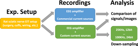
Figure 1. Workflow of in vivo data recording and analysis the present study. Electrophysiology setup is arranged and measurements are performed with commercial and custom current source. Resulting signals and images are compared. Signals from the custom system are subject to down-sampling analysis.
Download figure:
Standard image High-resolution imageA list of specifications can be set up to determine if quality of the modified system is only affected in negligible ways compared to the high-end ScouseTom setup:
- –Current source for nerve stimulation: Must be able to deliver pulses within amplitude and pulse width ranges typical for nerve stimulation (pulse width from 50 μS to few milliseconds, amplitude 0.25–5 mA); no meaningful pulse shape changes for resistive loads in the range from 0.5 KΩ to few KΩs; no meaningful pulse distortion due to capacitive loads up to 1 nF.
- –EIT Current source: Not noisier than existing commercial source in nerve EIT bandwidth during tank measurements.
- –ADC/Data acquisition board: Sampling rate should meet Shannon's criterion of 2× maximum frequency; for 6 KHz nerve measurements with 2 KHz bandwidth, 16 KHz is necessary. Sampling resolution should not add quantization noise to a level that increases post coherent-averaging noise to more than 1 μV, corresponding to ≈17 μV pre-averaging for the current number of averages.
2.2. New hardware design
Design of new hardware was performed with the guiding principle of providing the users with devices easy to use, simple to reprogram, and simple to modify. General device architecture for both boards was kept at the lowest possible level of complexity which guaranteed the desired performance. Power management was designed to allow power supply from either USB power banks or very common lithium-polymer (LiPo) 3.7 V batteries. Device control was performed with microcontroller boards based on the Arduino environment (https://arduino.cc) to allow easier communication and reprogramming by users. Specifically, the Seeduino XIAO (Seed Technology Inc., Shenzhen, China) was chosen as the smallest commercially available Arduino-based device (23.5 × 17.5 mm) to save board space. When possible, for similar functions requiring the same category of devices (e.g. operational amplifiers, switches), a single model of integrated circuit (IC) was chosen to take advantage of the existence of dual and quad IC packages and save board space. All resistors and capacitors were implemented as surface mount devices (SMD) with the SMD-0805 package size (2.0 × 1.2 mm). This package size was chosen as a compromise between saving board space and giving users with intermediate soldering skills the possibility to replace passive components to alter circuit gains and filter frequencies for their specific projects. All circuit design was performed in EAGLE (Autodesk, San Rafael, California, USA). Design files, including PCB Gerber files, and firmware code are available at https://github.com/EIT-team.
2.2.1. EIT current source (Sine-CS)
General architecture of the EIT current source is reported in figure 2(A) as a block diagram. Briefly, a voltage sine wave (VDDS) is generated by a discrete digital synthesis (DDS) device, band-pass filtered (VSin) and converted to current sine wave by a voltage-controlled current source (VCCS) circuit. Battery voltage (VBatt) is regulated before being supplied to the rest of the board. USB communication can be used to reprogram the output sine wave frequency but continuous USB communication is not necessary for board operation.
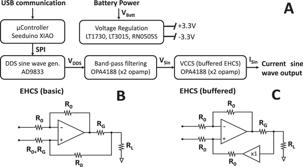
Figure 2. Architecture of the Sine-CS device and Howland circuit topologies. (A) Block diagram of the EIT current source board architecture. (B) Basic enhanced Howland current source architecture. (C) modified enhanced Howland current source architecture with buffering on the positive feedback branch.
Download figure:
Standard image High-resolution imagePower regulation was implemented by generating a dual voltage supply of ±3.3 V to power the analog and digital components of the device. Positive 3.3 V supply was generated by a fixed-output LT1763 regulator (Analog Devices, Wilmington, Massachusetts, USA). Negative 3.3 V supply was generated by inverting battery power using a DC-DC isolator (RN-0505S, RECOM power) and then regulating its output voltage to −3.3 V using a fixed-output LT3015 regulator (Analog Devices, Wilmington, Massachusetts, USA).
A reference voltage sine wave was generated using an AD9833 DDS IC (Analog Devices, Wilmington, Massachusetts, USA), connected to a generic SMD 25 MHz CMOS crystal oscillator with 50 ppm accuracy. Output frequency was set to be programmed into the DDS device from the microcontroller at power-up.
A quad-package operational amplifier IC, the OPA4188 (Texas Instruments, Dallas, Texas, USA) was used to implement voltage sine wave analog processing and voltage-to-current conversion. Analog processing was designed to implement bandpass filtering over the sine wave by performing low-pass filtering with a 2nd-order Sallen-Key architecture and a 33 KHz cut-off frequency, and high-pass filtering using a 1st-order passive filter with 15 Hz cut-off frequency. A buffer stage was implemented at filter output.
Voltage to current conversion was implemented using a buffered enhanced Howland current source (EHCS) circuit topology (Pease 2008, Xia et al 2019). The circuit diagram of this VCCS architecture is shown in figure 2(C), where R0 are fixed values resistors (typically 100 KΩ), RG is the gain-setting resistor, and RL is the equivalent resistor representing the circuit load, corresponding to the nerve tissue in our application. In this board, selection of current amplitude between four common values used for nerve EIT, 30–60–120–230 μA, was achieved by the use of manually selectable values for RG. In EHCS topologies, resistors on each branch of the circuit have to be matched to achieve theoretically infinite output impedance (Pease 2008). In the basic EHCS topology, shown in figure 2(B), this would lead to the requirement of switching two resistor values each time the gain setting is modified, corresponding to RG and R0 + RG in the figure. This number would increase to four in the case of a mirrored EHCS design (Bertemes-Filho et al 2012). The advantage of the buffered EHCS design in this regard, which led to its choice for this board, is that the presence of the buffer allows to disregard RG in matching the values of remaining resistors, all set to R0. Furthermore, all R0 resistors were implemented with 0.1% tolerance to minimize the effect of impedance mismatch. Thus, current amplitude can be modified by just changing RG value while not altering output impedance. Both operational amplifiers of the buffered EHCS are embedded in the same quad package of the OPA4188 and thus no extra board space is required for the buffered version compared to a traditional single op-amp EHCS topology.
2.2.2. Current pulse generator (Pulse-CS)
An overview of the architecture of the current pulse generator is shown in figure 3(A) as a block diagram. Briefly, a microcontroller unit receives current pulse settings (amplitude, frequency, mono/biphasic pulse) from a computer through USB connection. A digital-to-analog converter (DAC) communicates with the microcontroller through SPI protocol and is used to set pulse amplitude. Its output voltage (VCmd) is connected to a VCCS, based on an operational amplifier circuit shown in figure 3(B). Mono- and bi-phasic pulse generation (IPulse) is achieved by timed driving of electrical switches through digital I/O lines (DIO) to pilot the connection of the operational amplifier current output (ICmd) to the electrical load. Charge balance is achieved by shunting load terminals in-between pulses and in-between different phases of a biphasic pulses. Architecture of VCCS and switching protocol are based on the ReStore implantable stimulator (Sivaji et al 2019). Electrical isolation is present between the USB-connected microcontroller and the remaining circuitry which is battery-powered; since the microcontroller is non-isolated and USB-powered, continuous PC connection is required for operation. Pulse triggering can be achieved by an external digital signal, or pulse trains can be started by serial communication over USB. In figure 3(B), resistor RL represents the equivalent load of the electrodes and nerve connected to the device. Components R1, C1, RSet constitute a biasing network necessary for opamp stability, also adopted from the ReStore implantable stimulator.
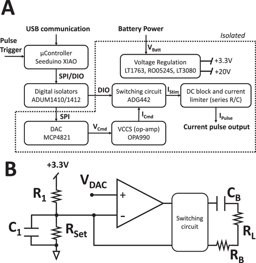
Figure 3. Architecture of the Pulse-CS device and topology of the voltage-to-current circuit. (A) Block diagram of the current pulse generator board architecture. (B) circuit diagram for the operational amplifier-based voltage-to-current converter used in this board.
Download figure:
Standard image High-resolution imagePower regulation was implemented by generating a positive voltage supply of +3.3 V to power the DAC and a +20 V voltage to power the VCCS and switching circuitry. Positive 3.3 V supply was generated by regulating battery power using a fixed-output LT1763 regulator (Analog Devices, Wilmington, Massachusetts, USA). Positive +20 V supply was generating by first up-converting battery voltage to +24 V using a DC-DC isolator (RO0524S, RECOM power) and then regulating the +24 V to a +20 V output using an LT3080 regulator (Analog Devices, Wilmington, Massachusetts, USA).
The MCP4821 (Microchip Technology, Chandler, Arizona, United States) was chosen as DAC for setting the pulse amplitude because of its 12bits resolution, internal 2.048 V voltage reference, and simple communication through SPI protocol.
An OPA990 (Texas Instruments, Dallas, Texas, USA) was chosen as the operational amplifier implementing voltage-current conversion for its high slew rate and capability for operating at high voltages.
Two ADG442 (Analog Devices, Wilmington, Massachusetts, USA) were chosen for implementing the switching circuitry capable of delivering monophasic and biphasic pulses for their short switching time and capability for operating at high voltages.
Digital isolation is achieved through components ADUM1410 and ADUM1412 (Analog Devices, Wilmington, Massachusetts, USA).
Safety features are implemented in the form of a DC current-blocking 1uF capacitor and a current-limiting 1 KΩ resistor, shows as CB and RB in figure 3(B). Both components are in series to the pulse circuitry output.
2.3. Preliminary circuit performance assessment
Performance of the Sine-CS and Pulse-CS devices was first assessed in fully controlled conditions before moving to in vivo experiments. For each testing effort which involved comparison with a benchtop device, the same current source as the ScouseTom system (model no. 6221, Keithley UK) was used.
For the Sine-CS EIT current source, performance was assessed with the following tests:
- (1)Current amplitude—Current injection was performed on resistive loads at all available current amplitude setting (figure 4(A)). Frequency was set at 6 KHz. Voltage measurements across the loads were performed with an oscilloscope. Sinusoidal traces recorded by the oscilloscope were exported to PC for post-processing. A sine-fitting algorithm (Ravagli et al 2020a) was used to detect amplitude, phase and DC offset of the recorded sine waves. Measured current amplitude values were compared to nominal values by computing average error and R2 correlation coefficient.
- (2)Noise levels—Current injection was performed in a tank filled with saline solution. Conductivity of saline solution was set to ∼0.3 S m−1, similar to conductivity of nerve tissue, and was prepared by dissolving NaCl (Sigma-Aldrich, St. Louis, Missouri, USA) in deionised water. Recordings of 2 min duration were performed with the Sine-CS device at all available current amplitude settings, and with the Keithley benchtop current source at matching current levels for comparison. A head tank was used due to availability but noise comparison between commercial and custom circuitry has general use which extends to nerve EIT. Current at 6 KHz was injected between two electrodes on opposing sides of the tank (see figure 4(B)). Voltage recordings were performed with an Actichamp EEG amplifier on electrodes adjacent to the injecting ones. Traces were demodulated with a ±1 KHz bandwidth around the EIT carrier and demodulated using the Hilbert transform. Noise was computed for each recording as the standard deviation of the demodulated amplitude signal. Noise levels computed from benchtop and custom current source recordings were compared by statistical analysis by performing a t-test between recordings taken at the same current amplitude.
- (3)Warm-up signal drift—Current injection was performed over a resistive load of 1.5 KΩ nominal value for a 40 min period of time with both current sources. Recordings were performed right after powering up each device to assess the time required for stabilisation of signal amplitude. Voltage signals across the resistor were recorded with an Actichamp EEG amplifier over an auxiliary channel and were demodulated as in previous test and were low-pass filtered with a 100 Hz cut-off frequency. Signal drift during device warm-up was evaluated as % variation from start to end of recording.For the Pulse-CS, performance was assessed with the following tests:
- (1)Pulse amplitude—Current pulses were delivered to a fixed load resistor of nominal 2.2 KΩ value (figure 4(C)). Pulse width was kept constant at 50 μs. Pulse amplitude was set to multiple values in the range of 250 μA–5 mA. Voltage drop across the load resistor was recorded for each amplitude value with an oscilloscope. Voltage recordings were normalised to effective current value by measuring the true resistor value. Measured current amplitude values were compared to nominal values by computing error and R2 correlation coefficient.
- (2)Load dependence—Current pulses of 2 mA amplitude and 50 μs duration were delivered to multiple resistive loads. Voltage drop across the load resistor was recorded for each resistor value with an oscilloscope. Voltage recordings were normalised to effective current value by measuring the true resistor value. Recorded pulses across the resistor were analysed by visual inspection in order to assess the presence of differences in pulse shape across different resistor values.
- (3)Pulse width—Current pulses were delivered to a fixed load resistor of nominal 2.2 KΩ value. Pulse amplitude was kept constant at 2 mA. Pulse width was set respectively to 0.5, 1 and 2 ms to evaluate capability of delivering long pulses. Voltage drop across the load resistor was recorded for each pulse width value with an oscilloscope. Measured pulse width values were compared to nominal values by computing error and R2 correlation coefficient.
- (4)Pulse symmetry—In all biphasic pulses from tests (1) to (3), difference between total charge of the positive and negative pulses was evaluated.
- (5)Capacitive load—Current pulses were delivered to a fixed load resistor of nominal 2.2 KΩ value connected in parallel to a load capacitor. Pulse amplitude was kept constant at 2 mA. Different capacitor values were explored to evaluate the capability of delivering pulses to loads with a reactive component. Capacitor values in the 10 pF–10 nF range were tested for a 50 μs pulse width. Capacitor values in the 10 pF–100 nF range were tested for a 500 μs pulse width. The voltage drop across the load resistor was recorded each time with an oscilloscope. Resulting pulse shapes were compared visually.
All oscilloscope recordings were performed with a mixed-signals oscilloscope (InfiniiVision MSOX3024T, Keysight); traces were sampled at 400 MHz and 12 bits resolution, then stored and exported to PC.
All EEG amplifier recordings were performed with an Actichamp EEG amplifier (Brain Products, Gilching, Germany) with 24 bits ADC resolution and ±400 mV signal range.
All post-processing was performed in MATLAB (MathWorks, Natick, USA). For all tests on all devices, realistic resistive loads have been simulated with through-hole resistors. Nominal values of resistors were 470 Ω, 1.5 KΩ, and 2.2 KΩ respectively. These values approximate the resistance of nerves ranging from rat sciatic nerve to pig vagus nerve. Real resistor values were measured using a high-precision benchtop multimeter (Model 34401A, Hewlett Packard) to improve accuracy of our performance assessment.
2.4. In vivo experiments
2.4.1. Physiological setup
The study was conducted in accordance with the European Commission Directive 2010/63/EU (European Convention for the Protection of Vertebrate Animals used for Experimental and Other Scientific Purposes) and the UK Home Office (Scientific Procedures) Act (1986) with project approval from the University College London Institutional Animal Care and Use Committee. In vivo experiments were performed as described previously (Aristovich et al 2018, Ravagli et al 2019, 2020b, 2021). Briefly, adult male Sprague-Dawley rats weighing 400–550 g were anesthetised with urethane (1.3 g kg−1, i.p.), intubated and artificially ventilated using a Harvard Apparatus Inspira Ventilator (Harvard Apparatus, Ltd, UK) with a 50/50% gas mixture of oxygen and air. Electrocardiogram and respiratory parameters (respiratory rate, end tidal CO2) were monitored (Cardiocap 5, Datex Ohmeda). The core body temperature of the animal was controlled with a homeothermic heating unit (Harvard Apparatus, Kent, UK) and maintained at 37°C. The animal was positioned prone, and the common sciatic nerve and its branches were dissected. The EIT cuff was placed around the main trunk of the sciatic nerve with the cuff opening facing superiorly and stimulation cuff electrodes (CorTec Gmbh, Freiburg, Germany) were placed around tibial and peroneal branches ∼1–1.5 cm distally from the EIT cuff. The surgical preparation from the moment of anesthesia onset to the beginning of recordings took on average 1 h. To avoid movement artifacts during recordings, neuromuscular blocking agent, pancuronium bromide (0.5 mg kg−1, i.m.) was used.
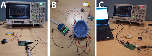
Figure 4. Preliminary testing of EIT sine wave current source and current pulse generator boards. (A) EIT sine wave current source testing on resistive loads. (B) evaluation of EIT current source noise levels in a tank. (C) pulse generator evaluation over load resistors.
Download figure:
Standard image High-resolution image2.4.2. EIT recordings
An overview of the FNEIT imaging pipeline is reported in figure 5.
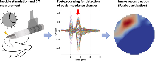
Figure 5. Fast neural EIT measurements in nerves. (A) EIT measurements are performed on a neural cuff while evoking responses from tibial or peroneal fascicles. (B) Raw data is post-processed to detect impedance changes as result of neural depolarisation. (C) Fascicle activation images are reconstructed from impedance changes.
Download figure:
Standard image High-resolution imageEIT measurements of fascicular neural traffic were performed with the ScouseTom system (Avery et al 2017) and its customized version. During these measurements, compound action potentials (CAPs) and impedance changes were evoked in fast myelinated (A-beta/delta) sensory/motor fibres in the tibial and peroneal fascicles of the sciatic nerve by delivering supramaximal biphasic pulse stimulation of individual branches at 20 Hz frequency and 50 μs pulse width with the CorTec cuffs bipolar electrodes. Current pulse amplitude was adjusted for each fascicle to maximize the magnitude ratio between the CAP and the stimulus artefact measured on the EIT cuff electrode array prior to EIT recordings, and was generally in the range of 200–1000 μA.
The electrode array cuff employed for recording surface CAPs and EIT data in rat sciatic nerve was the same design used in previous works by our group (Aristovich et al 2018, Ravagli et al 2019, 2020b, 2021). The cuff comprised two circumferential ring arrays of 14 electrodes, of which only one ring was used for cross-sectional current injections, with two reference electrodes placed at the extremities of the cuff. The cuff was made from silicone rubber spun onto 12.5 μm thick stainless steel foil, coated with PEDOT:pTS (Chapman et al 2019) and designed to wrap around the main trunk of a rat sciatic nerve with nominal 1.4 mm diameter. Post-coating electrode impedance was ∼1 KΩ, measured at 6 KHz.
For each nerve and fascicle, the EIT measurement were first performed with the original ScouseTom configuration, which employs commercial benchtop current sources (model no. 6221, Keithley UK), and then repeated with the customized system version developed in this work, which employs the compact current sources described in previous sections. The EIT protocol employed in this work comprised 14 transversal current injections with a skip-4 spacing drive pattern, corresponding to ∼100° on the cross-section of the nerve. This was previously identified by our group as one of the optimal protocols in terms of resolution (Ravagli et al 2019, 2020b). EIT current was injected at 6 KHz and 60 μA. Each current injection was 15 s long, leading to 300 repeated stimulation pulses at 20 Hz; thus, the total duration of the EIT measurement for each fascicle was 3.5 min.
2.4.3. Postprocessing and image reconstruction
Data from in vivo experiments were subject to the same general post-processing procedure from our previous work (Ravagli et al 2019, 2020b, 2021). Briefly, raw data were band-pass filtered with a ±2 KHz bandwidth around the 6 KHz EIT carrier and demodulated to voltage variations over time 'δ V' by extracting the amplitude of their Hilbert transform. Demodulated δ V traces were averaged over all the 300 repeated stimulation pulses to reduce noise and reach a SNR sufficiently high for successful EIT imaging. Some of the δ V traces were excluded from the reconstruction process based on the following criteria:
- DC saturation of raw signal, defined as the signal amplitude reaching the voltage range maximum of the EEG amplifier (±400 mV).
- High-noise traces, defined as post-averaging δV background noise >1.5 μV.
Image reconstruction was also performed similarly to previous work (Ravagli et al 2019, 2020b, 2021). Briefly, the UCL PEITS fast parallel forward solver (Jehl et al 2015) was used to compute solution to the EIT forward problem according to the complete electrode model (CEM). Rat sciatic nerve model geometry and mesh features were the same as in previous work cited above, including a forward mesh with 2.63 M elements and a reconstruction coarse hexahedral mesh with ∼75 K elements and 40 μm voxel size. Images were reconstructed by inversion of a coarse Jacobian matrix by 0th-order Tikhonov regularisation and noise-based voxel correction (Ventouras et al 2000, Aristovich et al 2018). For each reconstructed volume, one single cross-sectional slice was selected to act as reference image in the location with maximum reconstruction accuracy, as identified during optimization of our imaging protocol (Ravagli et al 2019). Image post-processing for quality enhancement was performed on selected 2D slices by median and mean filtering, both with a radius of 1-voxel distance from the voxel under analysis. Visualisation of reconstructed images was performed with Paraview (Kitware, New Mexico, USA).
For each recording, mean δ V and CAP amplitude were computed at peak time by averaging over all collected traces. Statistical analysis was performed to compare mean δ V and CAP amplitude recorded with the original and custom system.
2.5. Down-sampling analysis
To investigate the minimum required signal quality for imaging fascicular neural traffic, and the feasibility of performing nerve EIT using a recording module with lower specifications, raw data collected from the in vivo experiments using the customized version of the EIT recording system were artificially down-sampled in both resolution and sampling frequency. Raw data were originally collected with a sampling frequency of 100 KHz and an ADC resolution of 24 bits by the EEG amplifier comprised in the ScouseTom system. Data resolution was artificially lowered using a custom MATLAB (vR2018b, MathWorks, Natick, USA) script by performing the following steps:
- Low-pass filtering raw data with a 3rd-order Butterworth filter with 8 KHz cut-off frequency. This filter acts as a simulated anti-aliasing filter that would be embedded into the hardware of a recording module with lower sampling frequency.
- Down-sampling raw data to fractions of the original sampling frequency, while respecting Shannon's criterion for minimum sampling frequency.
- Reducing ADC resolution by approximating the value of each recorded data point to the nearest allowable value for a given resolution. An allowable value is defined as one of the 2N voltage values generated by quantization of the EEG amplifier voltage range (±400 mV) with N-bits resolution.
This process was repeated for a combination of 3 ADC resolution values (24, 16 and 12bits) and 3 sampling frequency values (100 KHz, 50 KHz and 25 KHz), thus generating a total of 9 simulated recording hardware specifications. The down-sampling process was performed on all data collected with the customized hardware, and the generated down-sampled recordings were processed with the same EIT post-processing method as the originals. For each recording, mean SNR was computed as the ratio between mean δ V at peak time and mean background noise, averaged over all traces. SNR percentage drop was computed as variation in mean SNR from original data sampled at 100 KHz, 24 bit.
Image reconstruction was performed over all recordings for a selected combination of down-sampled resolution and sampling frequency identified as the one with minimum acceptable SNR. Followingly, images reconstructed from original and down-sampled data were compared to evaluate the presence and magnitude of image quality loss as a result of the down-sampling process.
2.6. Statistical analysis and image comparison
All data in this work is reported as mean ±1 standard deviation, unless specified. Electrophysiology data (δ V, CAP) collected from the original and customized system were subject to a paired t-test for statistical analysis.
Image comparison for in vivo experiments (section 2.4) and down-sampling analysis (section 2.5) was performed according to three markers, by:
- Computing Centre of Mass (CoM) as in our previous work (Ravagli et al 2019) for each image and assessing distance between CoMs from images collected with each version of the system.
- Computing fascicle distinguishability, defined as distance between CoMs of tibial and peroneal fascicle, and comparing distinguishability between images collected with each version of the system.
- Computing R2 correlation factor over pixel-by-pixel intensity between images collected with each version of the system.
3. Results
3.1. Preliminary circuit performance results
Preliminary testing of the Sine-CS circuit showed capability of the circuit of delivering stable and accurate sinusoidal current waveforms. Amplitude of the delivered current sine wave, estimated by the fitting algorithm, was found to be on average −2.00 ± 1.39 μA lower than the set value. Correlation between set and measured values over the whole dataset was R2 > 0.99. Average DC values of the sine waves as estimated by the fitting algorithm were found to be 2.12 ± 0.34 mV. No statistical difference (p = 0.53) was found from the 2.05 mV value measured by shunting the oscilloscope probe, suggesting an offset in our recording instrument rather than in the Sine-CS circuit. An example of sine fitting result is shown in figure 6. Noise comparison over four current amplitudes returned average values of 1.68 ± 0.02 μV for the commercial current source and 1.61 ± 0.008 μV for the Sine-CS circuit, which proved statistically different (p = 0.0077). Sine-fitting and noise data are available in the supplementary material (available online at stacks.iop.org/PMEA/43/015004/mmedia), together with a figure showing the frequency spectra of the signals in the desired EIT bandwidth. Drift analysis (figure 7) showed that during a 40 min warm-up period, the commercial current source had a +0.32% amplitude variation, while the Sine-CS circuit only had a +0.26% variation.

Figure 6. Sine wave fitting. Example of sine fitting (red line) of data collected from the Sine-CS device (blue line) injecting current over a load resistor. Inset: details of the reconstructed sine wave.
Download figure:
Standard image High-resolution image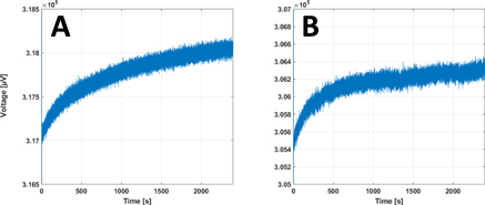
Figure 7. Drift at device warm-up. Drift in current amplitude during warm-up for commercial (A) and Sine-CS (B) current sources over 40 min.
Download figure:
Standard image High-resolution imageData collected from the Pulse-CS circuit preliminary testing indicated the capability of the circuit to deliver biphasic pulses of acceptable quality. Results from testing different pulse amplitude values (figure 8(A)) showed an average deviation from set values of −12 ± 43 μA, or −4.3 ± 5.8% of set value and a correlation of R2 > 0.99 between set and measured pulse amplitudes. Delivering pulses of 2 mA current amplitude over different resistive loads only resulted in minor pulse shape alterations on the lowest load of 470 Ω nominal value (figure 8(B)). Comparison of set and measured pulse widths (figure 9, plus 50 μs duration from figure 8, left) returned an average error of 2.0 ± 4.7 μs, or 2.3 ± 3.9%. Individual amplitude and pulse width values are reported in the supplementary material. Comparison of total charge over positive and negative components of the biphasic pulses returned a difference of 3.9 ± 3.6 nC, or 3.2 ± 2.9% of the positive component. Addition of a capacitive component to the stimulator load showed negligible alteration of pulse shape up to 1 nF when choosing a 50 μS pulse width (figure 8(C)) and up to 10 nF for 500 μS pulse width (figure 8(D)).
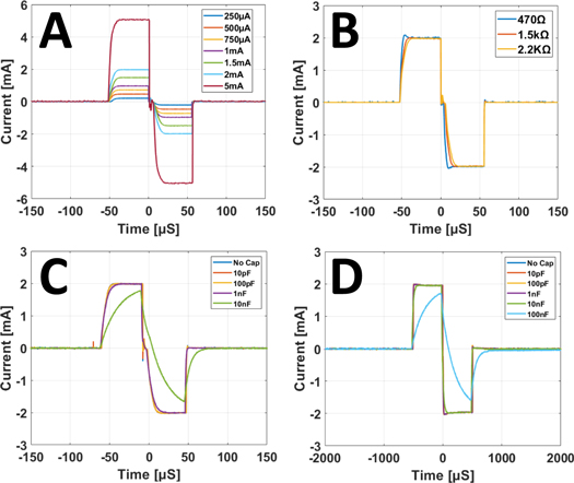
Figure 8. Characterisation of pulses for the Pulse-CS device. (A) biphasic pulses with pulse width of 50 μs delivered by the pulse-CS circuit over a resistive load of 2.2 KΩ nominal value at multiple current amplitudes. (B) Biphasic pulses with 50 μs pulse width and 2 mA current amplitude delivered over multiple resistive loads. (C) Biphasic pulse delivered with 50 μs pulse width, 2 mA amplitude, over a resistive load of 2.2 KΩ in parallel with multiple capacitive loads. (D) Same testing conditions as panel C, except for pulse width extended to 500 μs.
Download figure:
Standard image High-resolution image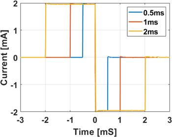
Figure 9. Testing of large pulse widths in the pulse-CS device. Current delivered at large pulse widths with 2 mA current amplitude over a resistive load of 2.2 KΩ nominal value.
Download figure:
Standard image High-resolution image3.2. In vivo results
EIT data were collected from three sciatic nerves from two rats. In each nerve, data were collected for tibial and peroneal fascicles. Each recording was repeated with both the ScouseTom system and the customized system. Thus, a total of N = 12 in vivo EIT recordings were performed. Evoked CAPs for tibial and peroneal fascicles had an average peak amplitude of 573 ± 287 μV and 487 ± 279 μV respectively for the original and customized system, with no statistically significant difference (t-test, p = 0.28). However, stimulation pulse amplitude needed to evoke supramaximal response in the individual fascicles was significantly higher (p = 0.043) for the Pulse-CS circuit compared to the commercial device (292 ± 252 μA versus 225 ± 284, respectively). EIT impedance traces collected from both fascicles had an average peak amplitude of 36 ± 14 μV and 31 ± 16 μV respectively for the original and customized system, with no statistically significant difference (t-test, p = 0.49). Data from individual recordings are reported in the supplementary material.
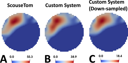
Comparisons of images reconstructed with the original and customized versions of the ScouseTom system from recordings performed in the same conditions, i.e. same fascicle, limb and animal (example in figures 10(A) and (B)) indicated a very high degree of similarity:
- The difference between CoMs of fascicular activation was found to be on average 37 ± 11 μm (<1voxel).
- Difference in fascicle distinguishability, i.e. distance between CoMs of tibial and peroneal fascicles in the same nerves, was 23 ± 17 μm (<1voxel).
- Pixel-by-pixel correlation between the images was R2 = 0.97 ± 0.02.
Figure 10. Image comparison. Example of images reconstructed from in vivo data collected using (A) commercial current sources, (B) our customized Sine-CS and Pulse-CS circuitry, and (C) down-sampled version of the data from the customized system (right).
Download figure:
Standard image High-resolution image
A comparison of all images reconstructed from the original ScouseTom system, the custom system, and the down-sampled dataset are available in the Supplementary material.
3.3. Down-sampling analysis results
Results from the down-sampling analysis of in vivo data, reported in table 1 as SNR and in table 2 as % reduction in SNR (ΔSNR%), show a cumulative SNR decrease with reduction in sampling frequency and ADC resolution.
Table 1. Average (±SD) SNR of original and down-sampled in vivo EIT data.
| SNR [-] | Resolution [Bits] | ||
|---|---|---|---|
| Fs [KHz] | 24 | 16 | 12 |
| 100 | 50.6 ± 20.9 | 50.1 ± 20.4 | 29.0 ± 11.5 |
| 50 | 44.5 ± 22.6 | 44.2 ± 22.3 | 26 ± 10.4 |
| 25 | 42.6 ± 23.0 | 42.4 ± 22.9 | 24.9 ± 10.0 |
Table 2. Average (±SD) % SNR reduction as an effect of down-sampling of in vivo EIT data.
| ΔSNR [%] | Resolution [Bits] | ||
|---|---|---|---|
| Fs [KHz] | 24 | 16 | 12 |
| 100 | 0.0 ± 0.0 | −0.9 ± 0.8 | −41.8 ± 11.1 |
| 50 | −14.7 ± 15.9 | −15.2 ± 15.6 | −48.5 ± 7.7 |
| 25 | −18.6 ± 19.6 | −18.9 ± 19.5 | −50.8 ± 7.2 |
The results above show that reducing sampling frequency, while keeping above the limit set by the Nyquist-Shannon sampling theorem, has an overall limited effect on SNR of the EIT impedance changes, less than 20% reduction with a four-fold reduction in sampling frequency down to 25 KHz, which is approximately three times the max frequency allowed by our anti-aliasing filter. Similarly, a very limited effect on SNR (<1%) can be observed when reducing ADC resolution from 24 bits to 16 bits at any sampling frequency, however a more marked drop is observed at 12 bits.
Based on these results, we identified the combination of 16 bits and 50 KHz as the threshold for down-sampling with acceptable SNR reduction. A comparison was performed between images reconstructed from the original, high-quality in vivo dataset and images reconstructed from data down-sampled with these parameters. The comparison, visually reported for one recording in figures 10(B) and (C), showed high consistency between the image sets:
- The difference between CoMs of fascicular activation was found to be on average 25 ± 22 μm (<1voxel).
- Difference in fascicle distinguishability, i.e. distance between CoMs of tibial and peroneal fascicles in the same nerves, was 20 ± 11 μm (<1voxel).
- Pixel-by-pixel correlation between the images was R2 = 0.99 ± 0.01.
4. Discussion
4.1. Results summary and answers to questions in 1.3
Overall, our study showed that our custom PCB circuitry was able to successfully replace the commercial current sources and deliver similar performances in both preliminary 'dry' testing and in vivo recordings, with the added values of compactness and low cost. Keithley-6221 current sources used in the ScouseTom setup are 104 × 238 × 370 mm in size, with a price of ≈£5000–6000 each, and evoked fast neural EIT requires two of them, one for nerve stimulation and one for EIT measurements. Dimensions of the developed boards are respectively ≈40 × 60 mm for Sine-CS and ≈50 × 78 mm for Pulse-CS. Both boards can be manufactured at a price of approximately £100 in total. In preliminary testing, our Sine-CS circuit was able to match, and slightly improve on, the noise and warm-up drift figures of the commercial current source when delivering 6 KHz EIT current (≈1.6 μV noise, ≈0.3% drift for both systems). Our Pulse-CS device proved able to deliver biphasic current pulses within a wide range of amplitudes and durations useful for evoking neural activity in small and large nerve fibres. During in vivo testing in three nerves, swapping from commercial to custom current source circuitry made no statistically significant difference in collected impedance changes and led to reconstruction to almost identical fascicular activation images (<40 μm difference in peak location, R2 = 0.97 pixel-by-pixel correlation). Regarding the down-sampling analysis, no large drop in SNR was detected (<20%) when lowering sampling rate two-fold to 50 KHz or four-fold to 25 KHz, and/or lowering ADC resolution to 16 bits. However, lowering ADC resolution further to 12bits proved the major factor for quality loss. Reconstructing images from data down-sampled at 16 bits, 50 KHz, no significant difference was detected compared to original images (<40 μm difference in peak location, R2 = 0.99 pixel-by-pixel correlation). Our modified system and simulated low-end ADC board satisfies the specifications set in section 2.1: the specifications for the nerve stimulator and EIT current source are satisfied by our Pulse-CS and Sine-CS devices. The specifications for the ADC are satisfied, in our down-sampling analysis, by 16bits and 25–50 KHz sampling rate. Overall, the results obtained from testing the newly developed devices and simulating lower sampling resolution suggest the possibility of dramatically decreasing the cost of the most expensive electronic modules and reduce the cost of a FNEIT system by a 30× factor down to <£1000.
A list of specifications can be set up to determine if quality of the modified system is only affected in negligible ways compared to the high-end ScouseTom setup:
- –Current source for nerve stimulation: Must be able to deliver pulses within amplitude and pulse width ranges typical for nerve stimulation (pulse width from 50 μS to 2 ms, amplitude 0.25–5 mA); no meaningful pulse shape changes for resistive loads in the range from 0.5 KΩ to few KΩs; no meaningful pulse distortion due to capacitive loads up to 1 nF.
- –EIT Current source: Not noisier than existing commercial source in nerve EIT bandwidth during typical tank measurements.
- –ADC/Data acquisition board: Sampling rate should meet Shannon's criterion of 2× maximum frequency; for 6 KHz nerve measurements with 2 KHz bandwidth, 16 KHz is necessary. Sampling resolution should not add quantization noise to a level that increases post coherent-averaging noise to more than 1 μV, corresponding to ≈17 μV pre-averaging for current number of averages.
The answers to the specific questions determined from this work are:
- (a)Can fast neural EIT be performed in nerves with compact and low-cost current source circuitry, without any loss of quality in collected data and reconstructed images?Yes, commercial high-end current sources can be replaced by compact and low-cost custom PCBs with no quality loss in fast neural nerve EIT.
- (b)Is a high-end recording system strictly necessary to detect fast neural changes in nerves or can more accessible lower-specifications hardware be used? If so, what are the minimum requirements?
Lower specifications down to a sampling rate of 25 KHz and an ADC resolution of 16 bits can be employed with no large repercussions on SNR when imaging evoked fascicular activity of healthy nerves, although a sampling frequency of 50 KHz is advised when possible. Requirements may be stricter in different conditions, e.g. unhealthy nerves or imaging of spontaneous activity.
4.2. Technical considerations
In this work, we adopted a version of the Howland voltage-to-current converter coupled to a DDS sine wave generator for delivering an EIT current sine wave. Several different architectures for voltage-to-current conversion exist, based around transistor, operational amplifiers, instrumentation amplifiers, or their combination. However, the chosen buffered EHCS circuit combines stability, accuracy and practicality and thus was ideal for implementing a simple but useful tool. While the general DDS + EHCS architecture of the Sine-CS was already investigated before in prior designs by our group (Dowrick et al 2015, Dowrick and Holder 2018), the Sine-CS devices offers improvements to voltage regulation, spectral purity and manual switching that overall justify the new design. The Sine-CS board is designed as a single-channel device, but multiple boards can be employed for parallel injections (Dowrick et al 2015, Dowrick and Holder 2018), provided that independent power supplies are employed. A particular point of interest of the preliminary testing results is that the noise level recorded with the Sine-CS board was almost identical to that of the commercial current source in a tank recording. This result may suggest that in the absence of biological noise generated by spontaneous neural activity, the current source noise is not the predominant contributor to total noise in the nerve EIT bandwidth, but rather the main contributors are the remaining electronic modules (switchboard and EEG amplifier) and environmental noise.
Our Sine-CS device was designed with cut-off frequencies of 15 Hz and 33 KHz respectively. This bandwidth is larger than required by nerve EIT, and was chosen to allow fast neural brain EIT (1.7 KHz), fast neural nerve EIT (6 KHz), stroke imaging (few Hz to 2 KHz) and to allow exploration above our current frequencies in future experiments, all without replacing components. However, having designed the device using SMD-0805 components, which can be hand-soldered, the passive filter element can also be replaced manually to tailor the bandwidth to specific user applications.
In this study, the Sine-CS device is evaluated either independently or in the context of a full in vivo nerve EIT experiment. In the future, it might be worthwhile to perform a more detailed investigation of the performance change, if any, induced by connecting the device to the electronic board used to implement injection pair switching in the EIT protocol. Presently, the positive results obtained from the in vivo experiments implicitly confirm that performance does not degrade significantly.
While the Sine-Cs device was designed to be a stand-alone hardware module able to operate with no continuous wired or wireless connection, the Pulse-CS device was designed with a continuous PC connection in mind. The main reason for this discrepancy is that the frequency and amplitude of EIT current is usually investigated apriori in dedicated sweep studies for each specific application and is fixed afterwards, thus the Sine-CS module only requires to be powered-up during an experiment. On the other hand, stimulation parameters like amplitude and pulse width needs to be modified several times to identify minimum supramaximal stimulation or to elicit activity in different types of fibres.
The new stimulator allows a larger voltage compliance of 20 V compared to the 12 V of the implantable ReStore device (Sivaji et al 2019), however, this value is still inferior to the nominal 100 V compliance of the Keithley 6221 benchtop devices. While this feature could be considered a limitation and addressed with additional steps of voltage up-conversion, it also limits the maximum amount of current which can be injected into the tissue and thus acts as an additional safety feature. With 20 V voltage compliance, 1 KΩ current-limiting resistor, and an expected tissue impedance in the range of 0.5–3 K KΩ, maximum injectable current lies in the range of 5–13 mA. This is abundantly sufficient in terms of amplitude for evoking activity from the fast myelinated fibres at the core of previous nerve EIT work, and also for evoking activity in larger myelinated or un-myelinated fibres typically targeted by neuromodulation efforts (Aristovich et al 2021). The asymmetry between positive and negative phases of the generated biphasic pulses proved to be very low and consistent with the amplitude and PW error figures (single-figure %) of the ReStore stimulator; more so, similarly to that device, charge balance in our Pulse-CS is also ensured by electrode shunting before, after and in-between pulse phases. Testing of the Pulse-CS device with different capacitive loads revealed only negligible alterations to pulse shape up to 1 nF for the shortest useful pulse width of 50 μS. With larger pulse widths, e.g. 500 μS, larger capacitive loads are also acceptable, since the effect of the reactive component is confined to the rise and fall times of the pulse. In case of necessity, the effect of excessive capacitive loads at short pulse widths can be compensated by setting a higher nominal current amplitude, or capacitive load can be decreased by performing PEDOT-coating of the stimulation electrodes.
Theoretically, the hardware of the Pulse-CS device can contribute to overall system noise when not administering a pulse, but in practice this contribution is limited by multiple factors. First, anode and cathode of the stimulator are shunted together in-between pulses to achieve charge balance. Secondly, the Pulse-CS device is not connected directly to the EIT recording system, except for a digital line sending pulse triggers, wired to the microcontroller prior to electrical isolation. Thirdly, Pulse-CS stimulates the nerve through a bipolar stimulation cuff which is physically separate from the EIT measurement cuff; thus, part of the noise will be filtered out by the low-pass properties of the tissue. The down-sampling analysis performed for this study showed, as expected, a progressive decrease in SNR when reducing sampling frequency and/or ADC resolution. This analysis presents a few key points deserving comment. The first point is that reducing ADC resolution from 24 to 16 bits, which corresponds to a 256-fold increase in quantization step, presents by itself only <1% drop in SNR, at each sampling frequency. The most likely explanation for this finding lies in the fact that raw data is subject to coherent averaging based on repeated stimulation pulses, and thus most of the additional quantisation noise is filtered out by this process. Another factor contributing to limiting the decrease in SNR is that quantisation noise is, statistically speaking, distributed over the entire raw signal bandwidth (Kester 2005) and only a fraction of it (2 KHz out of 25/50/100 KHz) is used as EIT bandwidth. However, further decrease in resolution to 12 bits leads to an excessive decrease in signal quality and thus is unacceptable as ADC resolution. This can be explained by the fact that with our recording module, a resolution of 24 bits over a signal range of ±400 mV corresponds to ≈47.7 nV quantization step; lowering the resolution to 16 bit leads to a quantization step of ≈12.2 μV, and lowering it to 12 bit leads to a ≈195 μV step. Thus, our impedance variations are already on the edge of detectability at 16 bits, but coherent averaging improves SNR to a level that allows the use of this resolution. With 12 bit, even SNR improvement from averaging is not sufficient for reaching imaging quality. Overall, this is not an issue for the design of a lower-specifications recording module, since 16 bits ADC with multiple parallel channels are widely diffused as commercial electronic components. The second point is that while the Sine-CS and Pulse-CS circuits proved fit for general future use in fast neural EIT experiment, the down-sampling analysis performed on a dataset collected for the rat sciatic nerve EIT experiment with evoked activity, and thus the identified threshold of 16 bits, 50 KHz for a lower-specifications recording module should only be considered valid for this specific type of protocol. Future aims of nerve EIT research include recoding signals from evoked activity over longer distances in large animals (e.g. 20 cm in pig rather than 2 cm in rat) or recording spontaneous signals where the benefit of coherent averaging on SNR improvement may be reduced or absent. In these cases, where SNR is expected to be lower compared to current conditions, the highest available resolution for sampling and quantization might still be required. More so, our third point is that in vivo experiments for this study were performed on very healthy nerves which led to recording of large evoked CAPs and impedance changes. Our evoked CAPs for tibial and peroneal fascicles have average peak amplitude of ≈500 μV, higher than the average ≈200–250 μV of the original work by Aristovich et al (2018) and average ≈180 μV of our previous work (Ravagli et al 2020b). In this work we reported impedance changes of ≈30–35 μV for tibial and peroneal fascicles, higher than the average ≈12 μV of our previous cross-validation work, in which nerves were injected with neural tracers and thus most likely subject to inflammation; lower impedance changes are to be expected on nerves subjected to chemical or mechanical stress and a lower starting SNR might be expected. These two last points indicate that results from our down-sampling analysis might not be extendable to every future fast neural EIT experiment but, nonetheless, they are encouraging in suggesting further possible device simplification. For more insight, we suggest performing future nerve EIT experiments in large animals with the same high-end ScouseTom setup and repeating the same down-sampling analysis.
In this study, quantitative comparison of images reconstructed from original versus customised system or before versus after down-sampling is performed by means of CoM and voxel-by-voxel correlation. Images of the same fascicular activation reconstructed in different conditions may result in similar CoMs and high R2 correlation while technically having different conductivity values; e.g. images in figure 10 have similar visual arrangement but different peak values. These differences can be explained with fluctuation in physiological status of the nerve between different recordings (figure 10(A) versus 10(B)) and by the effect of a lower SNR on our reconstruction algorithm (figure 10(B) versus 10(C)). Regardless of the source of conductivity range difference between images, we believe our metrics are optimal for assessing nerve EIT hardware performance since the location of the relative peak conductivity variation over the nerve's cross-section is the desired information for our target application, i.e. selective stimulation of fascicle groups.
While this work was aimed at improving circuitry for fast neural EIT of evoked nerve activity, the results can also be applied to brain EIT. EIT of brain activity was demonstrated experimentally (Aristovich et al 2016, Faulkner et al 2018, Hannan et al 2018, Hannan et al 2019) using current amplitude and frequency of the same order of magnitude as those used for nerve EIT (10–100 μA and 1.725 KHz for brain versus 30–200 μA and 6 KHz for nerve). As such, using the Sine-CS board for fast neural brain EIT would require minor or no adjustments. In the past, brain EIT was performed together with mechanical stimulation of whiskers (Aristovich et al 2016), for which an electrical stimulator was not needed, with electrical stimulation of the rat forepaw (Faulkner et al 2018) for fast activity, and with electrical stimulation of the somatosensory cortex used as an epilepsy model (Hannan et al 2018). For the last two cases, electrical stimulation was performed at 2 Hz, 500 μs, 10 mA and 100 Hz, 1 ms, 2 mA respectively, two sets of values achievable by the Pulse-CS board.
4.3. Limitations and future technical improvements
One limitation of the Pulse-CS found in this study regards delivery of correct amount of charge at lower current amplitudes. As reported in the result section, our custom stimulator required a statistically significantly higher current amplitude for evoking supramaximal CAPs compared to the commercial device. This value amounts to approximately +30% on average, but assessment on the individual values from different fascicles and nerves shows that the problem is mainly concentrated at low current amplitudes (<200 μA, see supplementary table S.T3). Our preliminary testing showed properly-timed delivery of even the shortest pulses, i.e. 50 μs, indicating that the problem is most likely associated to current amplitude rather than duration. The most likely explanation is that the presence of our DC-blocking capacitor and neural tissue capacitance leads to under-delivery of the set amount of charge at low amplitudes. This issue will be investigated and corrected in future iterations of the Pulse-CS board; however, it does not constitute a major limitation to its use. The amount of current amplitude needed for evoking supramaximal activity is based on multiple factors (size of the nerve, contact impedance, tightness of the cuff, etc) and has to be assessed iteratively each time with multiple CAP recording; thus, the user will not be required extra time to iterate the proper stimulation amplitude.
While the current design of the Sine-CS device only offers DC component minimization in the form of high-pass filtering of the voltage sine wave, additional DC removal can be achieved by adding a series DC-blocking capacitor to the output, similar to what was done for the Pulse-CS device.
One additional limitation of this study is that it is focused toward a specific single-frequency and narrow-band application; use of the developed circuitry, e.g. Sine-CS, for multifrequency and wideband EIT would require further frequency response and phase linearity analyses.
While the circuitry developed in this study offers a significant step in the direction of miniaturization and cost reduction for nerve EIT measurements, the overall architecture is still based on the pre-existing ScouseTom system, developed as a flexible and high-end system. Thus, control and switching circuitry still exist as separate modules in regard to the stimulation and EIT current sources. More so, while a down-sampling analysis indicated the feasibility of lower specifications for the recording module, a research high-end EEG recording system is still in use.
Future work will focus on integration of all the required modules into an embedded 'Nerve EIT board' ready for dissemination among neuroscience labs. While integration of control, switching and current source circuitry can be performed with moderate effort based on the existing open-source designs, implementation of a custom recording module will prove more challenging due to the need of managing parallel voltage recordings from multiple channels at high sampling frequency and resolution, i.e. high data collection and transfer rate. An embedded nerve EIT board will also need to account for electrical safety and would ideally feature wireless communication (e.g. Bluetooth) and low power consumption.
Acknowledgments
This work was supported by the UK Medical Research Council (MRC grant No: MR/R01213X/1) and NIH SPARC Program (grants 1OT2OD026545-01 and 3OT2OD025306-01S2).