

Abstract
Objectives. The human skeletal muscle responds immediately under electrical muscle stimulation (EMS), and there is an immediate physiological response in human skeletal muscle. Non-invasive quantitative analysis is at the heart of our understanding of the physiological significance of human muscle changes under EMS. Response muscle areas of human calf muscles under EMS have been detected by frequency difference electrical impedance tomography (fd-EIT). Approach. The experimental protocol consists of four parts: pre-training (pre), training (tra), post-training (post), and relaxation (relax) parts. The relaxation part has three relaxation conditions, which are massage relaxation (MR), cold pack relaxation (CR), and hot pack relaxation (HR). Main results. From the experimental results, conductivity distribution images σp (p means protocol = pre, tra, post, or relax) are clearly reconstructed by fd-EIT as response muscle areas, which are called the M1 response area (composed of gastrocnemius muscle) and the M2 response area (composed of the tibialis anterior muscle, extensor digitorum longus muscle, and peroneus longus muscle). A paired samples t-test was conducted to elucidate the statistical significance of spatial-mean conductivities 〈σp〉M1 and 〈σp〉M2 in M1 and M2 with reference to the conventional extracellular water ratio βp by bioelectrical impedance analysis. Significance. From the t-test results, 〈σp〉M1 and 〈σp〉M2 have good correlation with βp. In the post-training part, 〈σpost〉 and βpost were significantly higher than in the pre-training part (n = 24, p < 0.001). The relax–pre difference ratios of spatial-mean conductivity Δ〈σrelax–pre〉 and the relax–pre difference ratios of extracellular water ratio Δβrelax–pre in both MR and CR were lower; on the contrary, the Δ〈σrelax–pre〉 and Δβrelax–pre in HR were significantly higher than those in post–pre difference ratios of spatial-mean conductivity Δ〈σpost–pre〉 (n = 8, p < 0.05). The reason for the changes in 〈σp〉M1 and 〈σp〉M2 are caused by the changes in muscle extracellular volumes. In conclusion, fd-EIT satisfactorily evaluates the effectiveness of human calf muscles under EMS.
Export citation and abstract BibTeX RIS
1. Introduction
Electrical muscle stimulation (EMS) is an alternative method of voluntary exercise for people who are unable to perform high-intensity exercise (Banerjee et al 2005). EMS recruits muscle fibers quickly, even at lower forces (Bickel et al 2011), which causes an immediate physiological response and thereby changes in muscle extracellular volume (Fleckenstein et al 1988). In order to evaluate the effectiveness of EMS in situ, the electrical signal of human muscles under EMS between pre- and post-training should be detected because the electrical signal directly reflects the physiological response of muscle activity (Coggshall and Bekey 1970). Moreover, relaxation methods such as massage relaxation (Martin et al 1998), cold pack relaxation, and hot pack relaxation after EMS cause different physiological responses, which have good correlations with the flow rate changes of muscle tissue fluids (Cochrane 2004).
Generally, two muscle measurement methods are used to measure the physiological response of human muscle under EMS, which are the 'passive' measurement method of muscle electrical signals (Stulen and De Luca 1981) and the 'active' imaging method (Cagnie et al 2011) of injecting current into the muscles. In the passive measurement method, surface electromyography (sEMG) is typically used. The basic principle of sEMG is to detect the myoelectric signal generated from action potentials in contracted muscles. The time-frequency signals of sEMG quantitatively reflect the muscle functional status (Zhang et al 2011), muscle group coordination, and muscle strength (Hermens et al 2000). On the other hand, in the conventional active imaging method, computed tomography (CT), magnetic resonance imaging (MRI), and ultrasonic imaging (UI) are widely used to study the physiological characteristics of human muscles (Ito et al 1998). CT provides clear images of the muscle shape to distinguish muscle, fat, and bone accurately. MRI provides structural and functional muscle images of oxygenation (Partovi et al 2012) and contraction (Sinha et al 2004). It accurately reflects the muscle activity under EMS (Deligianni et al 2017). UI detects muscle thickness, muscle fiber plume angle, and muscle bundle activity (Lopata et al 2010).
However, the above conventional muscle measurement methods have drawbacks in evaluating the effectiveness of EMS in situ. For instance, sEMG is not able to image the localized response muscle areas of human muscle due to the excessive influence of noise (Son et al 2018). CT, MRI, and UI are not able to immediately detect the response muscle area under EMS because of vague morphological changes during a short period during the pre- and post-training and the relaxation parts. By contrast, electrical properties such as conductivity change in human muscles during the short period between pre- and post-training parts under EMS (Eriksson et al 1981). Under these circumstances, we have come up with an approach using electrical impedance tomography (EIT) (Yao and Takei 2017), which resolves the above-mentioned drawbacks to become a novel technique for detecting different response muscle areas under EMS.
EIT is a non-invasive, non-ionizing, fast-response, and inexpensive measurement technique in situ, which is able to image the internal conductivity distribution based on the boundary voltage–current data measured from the human body surface under different physiological conditions (Dowrick et al 2016). We have already applied a unique EIT called frequency difference electrical impedance tomography (fd-EIT) to detect flexible boundary shapes of bio-related objects with wearable sensors (Darma et al 2020). fd-EIT was also applied to heterogeneous imaging in subcutaneous adipose tissue due to physiological change by localizing abnormalities in the compartment (Ogawa et al 2020). Therefore, in this study, we have proposed fd-EIT for imaging response muscle areas of human muscles under EMS in situ, especially focusing on calf muscles. To the best of our understanding, this is the first time that EIT has been applied to detect response muscle areas of human muscles under EMS.
In order to evaluate the EIT as a visualization method of EMS, we can define the muscle area into the stimulated muscle area and the response muscle area. In post-training by EMS, the conductivity of the stimulated muscle area changes due to the change in muscle extracellular volumes, which is the physiological response of skeletal muscles to EMS stimulation. Based on a previous study (Gregory and Bickel 2005) and the results of this study, EMS only stimulates the superficial gastrocnemius of the calf. When the gastrocnemius is contracted, it will drive the tibialis anterior muscle, extensor digitorum longus muscle, and peroneus longus muscle to complete the tiptoe action. The repeated contraction of the gastrocnemius drives the tibialis anterior muscle, extensor digitorum longus muscle, and peroneus longus muscle to contract repeatedly, which also has a corresponding physiological response. According to this explanation, we consider the change in muscle extracellular volumes, tiptoe action, and repeated contractions as a physiological response. This physiological response is located in the response muscle area, which is monitored or visualized by EIT.
The objectives of this study are (1) to apply fd-EIT to image the response muscle areas of human calf muscles under EMS in pre-training, post-training, and relaxation parts, (2) to validate the reliability of the reconstructed conductivity distribution images σ p (p means protocol = pre, tra, post, or relax) by fd-EIT with comparison between the spatial-mean conductivity 〈σp 〉 and extracellular water ratio βp by bioelectrical impedance analysis (BIA), and (3) to discuss the statistical significance of 〈σp 〉 in response muscle areas in the pre-training, post-training, and relaxation parts by a paired samples t-test to evaluate the effectiveness of EMS and the three types of relaxation conditions.
2. Experiments
2.1. fd-EIT system and image reconstruction
Figure 1 shows the fd-EIT system composed of four units: a wearable sensor consisting of sixteen dry electrodes (Darma et al 2020), a digital multiplexer (made by Takei lab based on Arduino Due), an impedance analyzer (IM3570, HIOKI, Japan), and a PC including image reconstruction algorithm software. The impedance analyzer injects 1 mA sinusoidal current to the electrodes by the adjacent current injection method (Baidillah et al 2019) then measures the impedance Z by way of the digital multiplexer. The impedance analyzer has an impedance measurement accuracy of 0.08% and excitation frequency coverage from 4 Hz to 5 MHz.
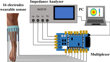
Figure 1. fd-EIT system.
Download figure:
Standard image High-resolution imageIn order to detect the response muscle areas of human calf muscles, the conductivity distribution images
σ
p
are reconstructed based on the theory of quasi-static electromagnetic field analysis (Gandhi et al
1993). In the forward problem, the Jacobian matrix is defined as J = [J1, J2,..., Jn
,..., JN
] 
 M×N
, where Jn
= [J1, J2,..., Jm
,..., JM
]T M
, m is the measurement number, n is the mesh number, M is the total measurement number, and N is the total pixel number of space resolution. The Jacobian matrix element Jmn
of the mth measured voltage pattern at the nth mesh element (Darma et al
2020) is obtained by
M×N
, where Jn
= [J1, J2,..., Jm
,..., JM
]T M
, m is the measurement number, n is the mesh number, M is the total measurement number, and N is the total pixel number of space resolution. The Jacobian matrix element Jmn
of the mth measured voltage pattern at the nth mesh element (Darma et al
2020) is obtained by

where u(ie ) is the potential field produced by injecting current i into the eth electrode, u(im ) is the potential field produced by injecting current i into the mth measured voltage pattern, vm is the measured voltage at the mth measured electrode pattern (1 ≤ m ≤ M), σn is the conductivity at the nth mesh (1 ≤ n ≤ N), and Ω is the electrical field area inside the fd-EIT sensor. J depends on the linearization of conductivity distribution in equation (1). In order to improve the accuracy of the reconstructed image, a modeled inhomogeneous conductivity distribution, which consists of bone (σbone = 0.020 S m−1), fat (σfat = 0.022 S m−1), and muscle (σmuscle = 0.321 S m−1) (Gabriel 1996), was used in the forward problem to calculate non-linear J.
Meanwhile, the inverse problem to reconstruct σ p from Z (Lionheart 2001) uses the Gaussian–Newton method (Darma et al 2020) expressed by

where μ is the hyperparameter which was chosen based on the error lying in the L-Curve's elbow (Braun et al
2017). ![${\rm{\Delta }}{{\bf{Z}}}^{p}=[{\rm{\Delta }}{Z}_{1}^{p},\ldots ,{\rm{\Delta }}{Z}_{m}^{p},\ldots ,{\rm{\Delta }}{Z}_{M}^{p}]$](https://content.cld.iop.org/journals/0967-3334/42/3/035008/revision4/pmeaabe9ffieqn1.gif)
 ℜM
is the impedance difference between one measured impedance Zp,f2 at high frequency f2 injection current and another measured impedance Zp,f1 at low frequency f1 injection current in fd-EIT (Baidillah et al
2017), which is expressed by
ℜM
is the impedance difference between one measured impedance Zp,f2 at high frequency f2 injection current and another measured impedance Zp,f1 at low frequency f1 injection current in fd-EIT (Baidillah et al
2017), which is expressed by

where p indicates the experimental protocol, which are pre-training (pre), training (tra), post-training (post), and relaxation (relax).
In this study, we focus on the muscle tissue located deeper in the skin and fat layer of the calf. As we all know, the contact impedance of the skin is very large, but for medical equipment, the injection current of EIT equipment cannot be higher than 1 mA. Therefore, we apply gel on the skin to reduce contact resistance. The reason for obtaining the best image from low frequency is that after EMS, the water content of the intercellular substance changes due to the effect of muscle congestion, and the high frequency directly mixes the intracellular information with the information obtained by the cell, so we believe that using a low frequency better reflects the changes in the moisture of the extracellular fluid. Therefore, two frequencies are heuristically selected as f1 = 700 Hz and f2 = 1 kHz to obtain the most clear σ p .
2.2. Experimental protocol and conditions
Twenty-four healthy young men (age: 30.0 ± 3.0 years, height: 173.5 ± 6.5 cm, skeletal muscle mass: 35.6 ± 6.8 kg) volunteered for this study. None of the subjects had any history of any musculoskeletal or neurological disorders. Figure 2 shows the experimental protocol consisting of four parts: pre-training, training, post-training, and relaxation parts (Zainuddin et al 2005). In all experimental protocols, subjects were measured in a sitting position.
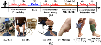
Figure 2. (a) Experimental protocol. (b) The specific steps in the experimental protocol using (i) fd-EIT, (ii) BIA, (iii) EMS, and relaxation methods of (iv) massage, (v) cold pack, and (vi) hot pack.
Download figure:
Standard image High-resolution imageIn the pre-training part, firstly, fd-EIT is conducted to reconstruct the conductivity distribution images σ pre in the human right calf; secondly, BIA (Inbody S10, InBody Co., Ltd, Korea) measures the extracellular water ratio βp = ECW/TBW, which is compared with the conductivity distribution change. Figure 3 shows the 16 electrodes of the fd-EIT sensor location and distribution.

Figure 3. fd-EIT sensor location and electrode distribution.
Download figure:
Standard image High-resolution imageIn the training and post-training parts, firstly, the subject's calf muscles are stimulated by EMS for 15 min using commercial EMS equipment (SIXPAD Leg belt, Nagoya MTG Ltd, Japan); secondly, fd-EIT is conducted to reconstruct the σ post in the human right calf; finally, BIA is used to measure βp . Figure 4 shows the position of the EMS electrode, which contacts the subject's skin directly. The EMS equipment in this study has a different voltage value but uses a constant-controlled current, which is 8 mA. The stimulation cycle rule is a 4 s stimulation with 4 s pause and the stimulation frequency is 20 Hz. After testing the EMS tolerance limit of each experimental subject, level 10 of EMS training intensity was selected from twenty training levels of EMS in situ. Level 10 means that the EMS output voltage is 26.13 V.

Figure 4. Electrode locations for electrical muscle stimulation.
Download figure:
Standard image High-resolution imageIn the relaxation part, the subjects' calf muscles were relaxed for 20 min by three methods of relaxation. The twenty-four subjects were divided into the massage relaxation (MR) group, cold pack relaxation (CR) group, and hot pack relaxation (HR) group with eight subjects per group. A water bag at around 12 °C was used to relax the subjects' calf muscles in the CR group. A towel soaked in hot water (temperature around 40 °C) was used to relax the subjects' calf muscles in the HR group. The temperatures of the water bag and towel were controlled by a temperature gun (the given error was ±5 °C). After relaxing, firstly, fd-EIT was conducted to reconstruct σ relax in the human right calf; finally, BIA was used to measure βp .
Due to the fd-EIT, the sensor needs to be taken off and worn repeatedly during the above-mentioned experimental protocol. Therefore, it was necessary to test the sensitivity of fd-EIT to displacement. Eight healthy young men (age: 29.6 ± 3.0 years, height: 175.0 ± 6.0 cm, skeletal muscle mass: 34.2 ± 6.2 kg) volunteered for this control group. Figure 3 shows the fd-EIT sensor position, which was marked with yellow tape. In the control group, firstly, fd-EIT was conducted to reconstruct the conductivity distribution images σ cg–pre in the human right calf; secondly, the subject was asked to wear the EMS for ten minutes, but the EMS was not switched on; then, fd-EIT was performed again to reconstruct the conductivity distribution image σ cg–post of the right calf. The above process was repeated twice for each subject.
2.3. Analysis method of response muscle areas
In order to quantify the response muscle areas of human calf muscles under EMS, the conductivity distribution images reconstructed by fd-EIT were analyzed by a dedicated Python script. Figure 5 shows an example of σ p of human calf muscles in the range of 0 < σ p ≤ 1.0 and the mesh structure used in this study. The mesh consists of 3053 trihedral element and 5263 points. In this paper, the view direction of σ p is from the top to the bottom of the human leg, which is contrary to the direction of typical CT images. Normally, the σ p indicates two response areas affected by EMS, which are denoted as M1 and M2 response areas. The conductivity values of M1 and M2 were changed in the pre-training, post-training, and relaxation parts. According to a typical MRI image of the calf muscle structure, M1 and M2 were calculated based on J by using the dedicated Python script in each subject. The reason why σ pre shows high conductivity in M1 and M2 before EMS is that the each subject's muscles have their own conductivity under the modeled inhomogeneous conductivity distribution in the forward problem. Therefore, σ pre was used as the baseline for each experimental subject in this study. The conductivity difference ratios Δ σ post– pre between pre- and post-training parts and Δ σ relax– pre between pre-training and relaxation parts are defined as


where the ⊘ symbol is the Hadamard division, which is the element-wise division of the column vector, and σ pre , σ post , and σ relax are the conductivity distribution images in the pre-training, post-training and relaxation parts, respectively.
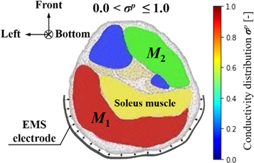
Figure 5. Example of conductivity distribution images σ p of human calf muscles.
Download figure:
Standard image High-resolution imageThe post–pre and relax–pre difference ratios of spatial-mean conductivity Δ〈σpost–pre 〉M1,M2 and Δ〈σrelax– pre 〉M1,M2 in M1 and M2 are defined as


where 〈σpre 〉M1,M2, 〈σpost 〉M1,M2, and 〈σrelax 〉M1,M2 are the spatial-mean conductivity in M1 and M2 in the pre-training, post-training, and relaxation parts. The conductivity distribution depends on the individual. In order to draw a general conclusion, we use the difference ratios to quantify the change in electrical conductivity distribution caused by the physiological response of post-training and relaxation of human muscles. Therefore, we proposed the application of fd-EIT to measure the effect of EMS on muscle training. In order to evaluate the difference ratios of spatial-mean conductivity, the post–pre and the relax–pre difference ratios of the extracellular water ratio Δβpost–pre and Δβrelax–pre are defined as


where βpre , βpost , and βrelax are the extracellular water ratios in the pre-training, post-training, and relaxation parts. The difference ratio quantifies the effects of post-training and relaxation of human muscles as references of Δ〈σpost–pre 〉M1,M2 and Δ〈σrelax–pre 〉M1,M2. The resolution of Inbody S10 is enough to calculate the percentage value, which can retain one digit after the decimal point (Masuda et al 2016).
2.4. Paired samples t-test
In order to use the paired samples t-test on the experimental data, it was necessary to perform a normal distribution test. The descriptive statistics function of SPSS software (version 25.0) was used to test the normal distribution of three parts of experimental data. Table 1 shows the results of the Shapiro–Wilk test and the Kolmogorov–Smirnov test. Under the test level of α = 0.05, p > 0.05, the null hypothesis is not rejected. Therefore, it can be considered that the experimental data obey a normal distribution.
Table 1. The results of the Shapiro–Wilk test and Kolmogorov–Smirnov test.
| Pre-training part | Post-training part | Relaxation part | ||||||||||||
|---|---|---|---|---|---|---|---|---|---|---|---|---|---|---|
| Kolomogorov–Smirnov | Shapiro–Wilk | Kolomogorov–Smirnov | Shapiro–Wilk | Kolomogorov–Smirnov | Shapiro–Wilk | |||||||||
| Condition | Items | df | Stats. | Sig. | Stats. | Sig. | Stats. | Sig. | Stats. | Sig. | Stats. | Sig. | Stats. | Sig. |
| Message relaxation | 〈σp 〉M1 | 8 | 0.286 | 0.053 | 0.890 | 0.234 | 0.241 | 0.190 | 0.871 | 0.153 | 0.247 | 0.163 | 0.840 | 0.076 |
| 〈σp 〉M2 | 8 | 0.194 | 0.200 | 0.950 | 0.716 | 0.193 | 0.200 | 0.898 | 0.278 | 0.201 | 0.200 | 0.929 | 0.510 | |
| βp | 8 | 0.216 | 0.200 | 0.904 | 0.315 | 0.227 | 0.200 | 0.907 | 0.331 | 0.213 | 0.200 | 0.895 | 0.261 | |
| Cold pack relaxation | 〈σp 〉M1 | 8 | 0.202 | 0.200 | 0.944 | 0.655 | 0.203 | 0.200 | 0.963 | 0.841 | 0.220 | 0.200 | 0.866 | 0.136 |
| 〈σp 〉M2 | 8 | 0.266 | 0.101 | 0.873 | 0.162 | 0.158 | 0.200 | 0.958 | 0.787 | 0.261 | 0.200 | 0.900 | 0.288 | |
| βp | 8 | 0.216 | 0.200 | 0.904 | 0.315 | 0.227 | 0.200 | 0.907 | 0.331 | 0.230 | 0.200 | 0.895 | 0.258 | |
| Hot pack relaxation | 〈σp 〉M1 | 8 | 0.247 | 0.163 | 0.889 | 0.228 | 0.197 | 0.200 | 0.913 | 0.378 | 0.182 | 0.200 | 0.934 | 0.554 |
| 〈σp 〉M2 | 8 | 0.168 | 0.200 | 0.957 | 0.785 | 0.134 | 0.200 | 0.957 | 0.784 | 0.200 | 0.200 | 0.834 | 0.065 | |
| βp | 8 | 0.141 | 0.200 | 0.963 | 0.836 | 0.172 | 0.200 | 0.914 | 0.382 | 0.153 | 0.200 | 0.938 | 0.595 | |
A paired samples t-test was conducted between the spatial-mean conductivities 〈σp 〉M1,M2 in the M1 and M2 response areas in order to elucidate the response muscle areas of human calf muscles under EMS and after relaxation. Also, the t-test is conducted in the extracellular water ratio βp for the evaluation. The test statistic t-values of the paired samples t-test are calculated by

where  is the mean difference of the experimental subject number n, and Sdiff
is the standard deviation of the differences. The level of significance was set as 0.05. The paired samples t-test was performed using SPSS software (version 25.0).
is the mean difference of the experimental subject number n, and Sdiff
is the standard deviation of the differences. The level of significance was set as 0.05. The paired samples t-test was performed using SPSS software (version 25.0).
3. Experimental results
3.1. fd-EIT sensor displacement sensitivity test
Table 2 shows the conductivity distribution images σ cg–pre and σ cg–post of eight subjects' calves before and ten minutes after wearing the EMS sensor obtained by equation (2). From σ cg–pre and σ cg–post , the M1 and M2 areas have no significant difference in two-times measurements. Also, figure 6 shows the spatial-mean conductivity 〈σcg–pre 〉M1,M2 and 〈σcg–post 〉M1,M2. The spatial-mean conductivity in M1 remains unchanged from 〈σcg–pre 〉M1 = 0.159 to 〈σcg–post 〉M1 = 0.160 in the first measurement; also, in the second measurement, the spatial-mean conductivity in M1 remains unchanged from 〈σcg–pre 〉M1 = 0.158 to 〈σcg–post 〉M1 = 0.157. The spatial-mean conductivity in M2 holds stable between 〈σcg–pre 〉M2 = 0.052 and 〈σcg–post 〉M2 = 0.055 in the first measurement; similarly, the spatial-mean conductivity in M2 holds stable between 〈σcg–pre 〉M2 = 0.054 and 〈σcg–post 〉M2 = 0.054 in the second measurement. Therefore, we conclude that only wearing the fd-EIT sensor repeatedly has no significant effect on the conductivity distribution measurement results.
Table 2. Conductivity distribution images σ cg–pre and σ cg–post before and ten minutes after wearing EMS sensor reconstructed by fd-EIT.
|

Figure 6. 〈σcg 〉M1 paired samples t-test results between before and ten minutes after wearing the EMS sensor for different subjects in control group. (b) 〈σcg 〉M2 paired samples t-test results before and ten minutes after wearing the EMS sensor for different subjects in control group.
Download figure:
Standard image High-resolution image3.2. Pre- and post-training parts
Table 3 shows the conductivity distribution images σ pre and σ post of twenty-four subjects' calves in pre- and post-training parts obtained by equation (2), and the conductivity difference ratios Δ σ post– pre between pre- and post-training parts obtained by equation (4). From the σ pre and σ post , the response muscle areas are clearly detected in the M1 and M2 response areas. Also, from the images Δ σ post–pre , the conductivity difference ratios between pre- and post-training parts in the response muscle areas are clearly detected.
Table 3. Conductivity distribution images σ pre and σ post in pre- and post-training parts reconstructed by fd-EIT and the conductivity difference ratios Δ σ post– pre.
|
Solid color bar charts in figure 7 show the spatial-mean conductivity 〈σpre 〉M1,M2 and 〈σpost 〉M1,M2 in M1 and M2 and extracellular water ratio βpre and βpost in the pre- and post-training parts. Dot color bar charts in figure 7 show the difference ratio of spatial-mean conductivity Δ〈σpost–pre 〉M1,M2 in M1 and M2 response areas between pre- and post-training parts. The spatial-mean conductivity in M1 is increased from 〈σpre 〉M1 = 0.194 to 〈σpost 〉M1 = 0.504 by Δ〈σpost–pre 〉M1 = 173.0%; also, the spatial-mean conductivity in M2 is increased from 〈σpre 〉M2 = 0.071 to 〈σpost 〉M2 = 0.182 by Δ〈σpost–pre 〉M2 = 174.6%. These increase tendencies are similar to the extracellular water ratio from βpre = 0.369 to βpost = 0.378 by the difference ratio between pre- and post-training parts Δβpost–pre = 2.3%.

Figure 7. (a) 〈σp 〉M1 paired samples t-test results between pre- and post-training parts and Δ〈σpost 〉M1 of different subjects between pre- and post-training parts. (b) 〈σp 〉M2 paired samples t-test results between pre- and post-training parts and Δ〈σpost 〉M2 of different subjects between pre- and post-training parts. (c) βp paired samples t-test results between pre- and post-training parts and Δβpost of different subjects between pre- and post-training parts. * p <0.05, ** p <0.01.
Download figure:
Standard image High-resolution imageTable 4 shows the statics of paired samples t-test in the pre- and post-training parts. The null hypotheses in 〈σp
〉M1, M2 areas are rejected because t-values tM1 = −10.452 and tM2 = −9.987 are smaller than -t0.025 (23) = −2.069. We conclude that 〈σpost
〉M1, M2 are significantly increased from 〈σpre
〉M1, M2 in both response areas. Moreover, the null hypothesis in the extracellular water ratio βp
is rejected because tβ
= −9.529 is smaller than t0.025(23) = −2.069. We conclude that βpost
is significantly increased from βpre
. The mean difference  of βpost
is −0.0085 (n = 24, p < 0.001) in the post-training part. The bottom row in table 4 and above-mentioned figure 7 show the p-value of 〈σp
〉M1,M2 in the paired samples t-test results between the pre- and post-training parts, which have the same tendency as the p-value of βp
.
of βpost
is −0.0085 (n = 24, p < 0.001) in the post-training part. The bottom row in table 4 and above-mentioned figure 7 show the p-value of 〈σp
〉M1,M2 in the paired samples t-test results between the pre- and post-training parts, which have the same tendency as the p-value of βp
.
Table 4. Statics of paired samples t-test of 〈σp 〉M1,M2 and βp (p = pre or post) between pre- and post-training parts.
| Items | 〈σp〉M1 | 〈σp〉M2 | βp |
|---|---|---|---|
Mean difference 
| −0.3106 | −0.1109 | −0.0085 |
| Standard deviation Sdiff | 0.1456 | 0.0544 | 0.0044 |
| t0.025(23) | −2.069 | ||
| t-value | −10.452 | −9.987 | −9.529 |
| p-value | <0.001 | <0.001 | <0.001 |
3.3. Relaxation part
Table 5 shows the conductivity distribution images 
 , and
, and  of the experimental subjects' calves under the three relaxation conditions (MR, CR, and HR) obtained by equation (2). Also, table 5 shows the conductivity difference ratios
 , and
, and  between the pre-training and relaxation parts obtained by equation (5). From
 , and
, and  the response muscle areas are also clearly detected in M1 and M2. From
 , and
, and  the conductivity difference ratios between the pre-training and relaxation parts in the response muscle areas are clearly detected.
Table 5. Conductivity distribution images σ relax in relaxation part reconstructed by fd-EIT and the conductivity difference ratios Δ σ relax–pre .
|
Solid color bar charts in figure 8 show the spatial-mean conductivity 〈σrelax 〉M1,M2(MR,CR,HR) in M1 and M2 in the relaxation part as well as 〈σpost 〉M1,M2 in the post-training part for the below-mentioned discussion. The dot color bar charts in figure 8 show the difference ratio of spatial-mean conductivity Δ〈σrelax–pre 〉M1,M2(MR,CR,HR) in M1 and M2 between the pre-training and relaxation parts.

Figure 8. (a) 〈σp 〉M1 paired samples t-test results between post-training and relaxation parts and Δ〈σpost 〉M1 of different subjects between post-training and relaxation parts. (b) 〈σp 〉M2 paired samples t-test results between post-training and relaxation parts and Δ〈σpost 〉M2 of different subjects between post-training and relaxation parts. (c) βp paired samples t-test results between post-training and relaxation parts and Δβpost of different subjects between post-training and relaxation parts. *p<0.05, **p<0.01.
Download figure:
Standard image High-resolution imageIn MR, the spatial-mean conductivity in M1 is decreased from 〈σpost
〉M1 = 0.504 to 〈σrelax
〉M1(MR) = 0.261 by Δ〈σrelax–pre
〉M1(MR) = 29.5%; also, the spatial-mean conductivity in M2 is decreased from 〈σpost
〉M2 = 0.182 to 〈σrelax
〉M2(MR) = 0.115 by Δ〈σrelax–pre
〉M2(MR) = 40.4%. This decrease tendency is similar to the extracellular water ratio from βpost
= 0.378 to  = 0.372 by the difference ratio between pre-training and relaxation parts
  = 0.5%.
In CR, the spatial-mean conductivity in M1 is decreased from 〈σpost
〉M1 = 0.504 to 〈σrelax
〉M1(CR) = 0.241 by relax–pre ratio Δ〈σrelax–pre
〉M1(CR) = 23.9%; also, the spatial-mean conductivity in M2 is decreased from 〈σpost
〉M2 = 0.182 to 〈σrelax
〉M2(CR) = 0.088 by relax–pre ratio Δ〈σrelax–pre
〉M2(CR) = 26.5%. This decrease tendency is similar to the βpost
= 0.378 to  = 0.371 by the difference ratio between pre-training and relaxation parts
  = 0.4%.
However, in HR, the spatial-mean conductivity in M1 is increased from 〈σpost
〉M1 = 0.504 to 〈σrelax
〉M1(HR) = 0.621 by Δ〈σrelax–pre
〉M1(HR) = 258.6%; also, the spatial-mean conductivity in M2 is increased from 〈σpost
〉M2 = 0.182 to 〈σrelax
〉M2(HR) = 0.207 by Δ〈σrelax–pre
〉M2(HR) = 268.1%. This decrease tendency is similar to the βpost
= 0.378 to  = 0.379 by the difference ratio between pre-training and relaxation parts
  = 3.0%.
Table 6 shows the statics of the paired samples t-test under three relaxation conditions. In MR, the null hypotheses in 〈σrelax
〉M1,M2(MR) areas are rejected because
t-
values tM1(MR) = 7.216 and tM2(MR) = 7.385 are larger than t0.025(7) = 2.365. We conclude that 〈σrelax
〉M1,M2(MR) is significantly decreased from 〈σpost
〉M1,M2 in both response areas. Moreover, the null hypothesis in the  is rejected because tβ(MR) = 4.492 is larger than t0.025(7) = 2.365. We conclude that
  is significantly decreased from βpost
. The mean difference
is significantly decreased from βpost
. The mean difference  of
of  is 0.0070 (n = 8, p < 0.05) in MR. In CR, the null hypotheses in 〈σrelax
〉M1,M2(CR) areas are rejected because
t-
values tM1(CR) = 5.269 and tM2(CR) = 5.960 are larger than t0.025(7) = 2.365. We conclude that 〈σrelax
〉M1,M2(CR) is also significantly decreased from 〈σpost
〉M1,M2 in both response areas. Moreover, the null hypothesis in the
is 0.0070 (n = 8, p < 0.05) in MR. In CR, the null hypotheses in 〈σrelax
〉M1,M2(CR) areas are rejected because
t-
values tM1(CR) = 5.269 and tM2(CR) = 5.960 are larger than t0.025(7) = 2.365. We conclude that 〈σrelax
〉M1,M2(CR) is also significantly decreased from 〈σpost
〉M1,M2 in both response areas. Moreover, the null hypothesis in the  is rejected because tβ(CR) = 5.314 is larger than t0.025(7) = 2.365. We conclude that
  is significantly decreased from βpost
. The mean difference
is significantly decreased from βpost
. The mean difference  of
of  is 0.0073 (n = 8, p < 0.05) in CR.
Table 6. Paired samples t-test results of the 〈σp 〉M1,M2 and βp between post-training and relaxation parts.
| Items | 〈σp〉M1 | 〈σp〉M2 | βp | ||||||
|---|---|---|---|---|---|---|---|---|---|
| MR | CR | HR | MR | CR | HR | MR | CR | HR | |
Mean difference 
| 0.2602 | 0.3117 | −0.1816 | 0.1013 | 0.0980 | −0.0626 | 0.0070 | 0.0073 | −0.0028 |
| Standard deviation Sdiff | 0.1020 | 0.1673 | 0.1230 | 0.0388 | 0.0465 | 0.0382 | 0.0044 | 0.0039 | 0.0033 |
| t0.025(7) | 2.365 | ||||||||
| t-value | 7.216 | 5.269 | −4.177 | 7.385 | 5.960 | −4.635 | 4.492 | 5.314 | −2.392 |
| p-value | <0.001 | 0.001 | 0.004 | <0.001 | <0.001 | <0.05 | 0.003 | 0.001 | 0.048 |
However, in HR, the null hypotheses in 〈σrelax
〉M1,M2(HR) areas are rejected because t-values tM1(HR) = −4.177 and tM2(HR) = −4.635 are smaller than -t0.025(7) = −2.365. We conclude that 〈σrelax
〉M1,M2(HR) is significantly increased from 〈σpost
〉M1,M2 in both response areas. Moreover, the null hypothesis in the  is rejected because tβ(HR) = −2.392 is smaller than -t0.025(7) = −2.365. We conclude that
  is significantly increased from βpost
. The mean difference
is significantly increased from βpost
. The mean difference  of
of  is −0.0028 (n = 8, p < 0.05) in HR. The bottom row in table 5 and above-mentioned figure 8 show the p-value of 〈σp
〉M1,M2 in the paired samples t-test results between the post-training and relaxation parts, which have the same tendency of the p-value of βp
. Therefore, the conductivity change of human calf muscles under different relaxation conditions is related to the muscle tissue fluid.
is −0.0028 (n = 8, p < 0.05) in HR. The bottom row in table 5 and above-mentioned figure 8 show the p-value of 〈σp
〉M1,M2 in the paired samples t-test results between the post-training and relaxation parts, which have the same tendency of the p-value of βp
. Therefore, the conductivity change of human calf muscles under different relaxation conditions is related to the muscle tissue fluid.
4. Discussion
4.1. Conductivity change from viewpoint of muscle extracellular volumes
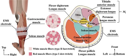
Firstly, the reason why the conductivities of human calf muscles under EMS in the M1 and M2 response areas are increased in the post-training part is discussed. Generally, two types of skeletal muscle fibers exist in human muscles, which are white muscle fibers (type II fast-twitch) and red muscle fibers (type I slow-twitch). When EMS is applied to human muscles, stimulation current induces an eccentric contraction of muscles (Lepley et al 2015). EMS quickly recruits white muscle fibers for contraction (Sinacore et al 1990), which generates high explosive power. The red muscle fibers are mainly used for long-term aerobic exercises (Stuart et al 2013).
Figure 9 shows the human calf muscle structure and cross-sectional image. From this figure, M1 is recognized as the position of the gastrocnemius muscle. From a previous electromyography study, the gastrocnemius muscle is recognized to be primarily involved in the fast movements of the leg as it is dominated by white muscle fibers (Mademli and Arampatzis 2005). Therefore, the conductivity 〈σpost 〉M1 in M1 is increased in the post-training by gastrocnemius muscle contraction.
Figure 9. Human calf muscle structure and cross-sectional image.
Download figure:
Standard image High-resolution image
Moreover, M2 is recognized as the position of the tibialis anterior muscle, extensor digitorum longus muscle, and peroneus longus muscle. From the viewpoint of muscle structure, these muscles in M2 on the front calf side are stretched while the gastrocnemius muscle is contracted because those muscles of M1 and M2 work together to make the tiptoe movement. The muscles in M2 are also trained simultaneously even though M2 is not covered by EMS while the gastrocnemius muscle is repeatedly contracted under EMS. Therefore, the spatial-mean conductivity 〈σpost 〉M2 in M2 is also increased in the post-training part.
Secondly, why soleus muscles are not responded by EMS is discussed even though the posterior calf muscles are mainly composed of gastrocnemius muscles and soleus muscles. From figure 9, the soleus muscles located behind the gastrocnemius (farther from the skin) have more red muscle fibers, and are the primary active muscles in a standing posture. While EMS is applied to human calf muscles, the stimulation current does not cause soleus muscle contraction in a short time. In addition, a more recent study has shown that EMS only indiscriminately stimulates the most superficial muscle fibers under the electrodes (Gregory and Bickel 2005). The soleus muscles is located behind the gastrocnemius (farther from the skin). In short, the deep soleus muscle cannot be stimulated by EMS. Therefore, the conductivity in the soleus muscle position is not changed in the post-training part.
Thirdly, the reason why conductivities are increased in M1 and M2 is discussed from the viewpoint of the change in muscle tissue extracellular volumes. Fleckenstein et al first reported that T2-weighted active skeletal muscle spin-echo MRI images showed increased signal intensity immediately after EMS training (Fleckenstein et al 1988). This phenomenon has also been studied in other research (Fisher et al 1990). It was proposed that this contrast enhancement of the exercised muscle was caused by increased vascular and extracellular volumes (Fleckenstein et al 1988). Therefore, the change in muscle tissue extracellular volumes is used to determine whether the target muscles are trained effectively. Compared with the pre-training part, the greater βp recorded in the post-training part is reasonable, since much water is transported to the muscle, causing muscle tissue fluid to increase. Therefore, the spatial-mean conductivity 〈σp 〉M1,M2 of human calf muscles increase.
4.2. Correlation between electrical conductivity and muscle tissue fluid
The reason why the conductivities of human calf muscles in M1 and M2 response areas have different changes under the three relaxation conditions is discussed.
In MR, 〈σrelax
〉M1,M2(MR) is decreased from 〈σpost
〉M1,M2 while  decreases from βpost
because MR promotes the removal of metabolites such as lactic acid and H+ from the muscle tissues. Massage increases the movement of lymphatic fluid and blood, facilitating their transfer to gluconeogenic organs such as the liver (Stamford et al
1981). Therefore, MR effectively reduces the concentration of muscle cell metabolites, thereby alleviating muscle extracellular volumes in the post-training part.
decreases from βpost
because MR promotes the removal of metabolites such as lactic acid and H+ from the muscle tissues. Massage increases the movement of lymphatic fluid and blood, facilitating their transfer to gluconeogenic organs such as the liver (Stamford et al
1981). Therefore, MR effectively reduces the concentration of muscle cell metabolites, thereby alleviating muscle extracellular volumes in the post-training part.
In CR, 〈σrelax
〉M1,M2(CR) is decreased from 〈σpost
〉M1,M2 while  decreases from βpost
because CR decreases muscle temperature (Enwemeka et al
2002). The decrease in muscle tissue temperature is thought to stimulate the cutaneous receptors, causing the sympathetic fibers to vasoconstrict, which decreases the muscle extracellular volumes (Pugh et al
1955).
decreases from βpost
because CR decreases muscle temperature (Enwemeka et al
2002). The decrease in muscle tissue temperature is thought to stimulate the cutaneous receptors, causing the sympathetic fibers to vasoconstrict, which decreases the muscle extracellular volumes (Pugh et al
1955).
In HR, the 〈σrelax
〉M1,M2(HR) are increased from 〈σpost
〉M1,M2 while  increases from βpost
because HR increases muscle tissue temperature, local blood flow, and muscle elasticity and causes local vasodilation (Pugh et al
1955). Therefore, the conductivity distribution change of human calf muscles under EMS is related to muscle extracellular volumes, which has been detected by frequency difference electrical impedance tomography (fd-EIT).
increases from βpost
because HR increases muscle tissue temperature, local blood flow, and muscle elasticity and causes local vasodilation (Pugh et al
1955). Therefore, the conductivity distribution change of human calf muscles under EMS is related to muscle extracellular volumes, which has been detected by frequency difference electrical impedance tomography (fd-EIT).
5. Conclusions
The present study reveals that response muscle areas of human calf muscles under EMS have been detected by fd-EIT. The key findings of this study are as follows.
- (1)Based on the reconstructed images, fd-EIT satisfactorily detects the physiological response areas of human calf muscles under EMS in pre-training, post-training, and relaxation parts.
- (2)In the post-training part, the spatial-mean conductivity 〈σpost 〉M1,M2 increases as the muscle extracellular volumes increases. In MR and CR, 〈σrelax 〉M1,M2(MR,CR) decreases as the extracellular water decreases due to massage facilitating blood circulation. Therefore, the conductivities in the M1 and M2 response areas are restored to those in the pre-training part. However, HR increases 〈σrelax 〉M1,M2(HR) by causing vasodilation.
- (3)The paired samples t-test results of this investigation demonstrate that in the detection of the muscle response areas of each pair of comparison populations, the p-value of 〈σp 〉M1,M2 is smaller than 0.05; therefore, 〈σp 〉M1,M2 is considered to be statistically significant.
Acknowledgments
The authors would like to thank Mr Prima Asmara Sejati and Mr Kaname Ikeda of Chiba University for their assistance with the experiments. They also thank Mr Martin Sifuna for his help in editing the final manuscript.
Ethical approval and informed consent
According to Chiba University ethical code, all subjects gave written informed consent for the study after receiving a detailed explanation of the purposes, potential benefits, and risks associated with participation. All study procedures were conducted in accordance with the Declaration of Helsinki and research code of ethics of Chiba University, and were approved by the Committee for Human Experimentation of Chiba University. The ethical approval number for our experiments by the Committee of Human Experimentation of Chiba University is 29-13.