
Abstract
Objective. In this study, we tackle the challenge of latency in magnetic resonance linear accelerator (MR-Linac) systems, which compromises target coverage accuracy in gated real-time radiotherapy. Our focus is on enhancing motion prediction precision in abdominal organs to address this issue. We developed a convolutional long short-term memory (convLSTM) model, utilizing 2D cine magnetic resonance (cine-MR) imaging for this purpose. Approach. Our model, featuring a sequence-to-one architecture with six input frames and one output frame, employs structural similarity index measure (SSIM) as loss function. Data was gathered from 17 cine-MRI datasets using the Philips Ingenia MR-sim system and an Elekta Unity MR-Linac equivalent sequence, focusing on regions of interest (ROIs) like the stomach, liver, pancreas, and kidney. The datasets varied in duration from 1 to 10 min. Main results. The study comprised three main phases: hyperparameter optimization, individual training, and transfer learning with or without fine-tuning. Hyperparameters were initially optimized to construct the most effective model. Then, the model was individually applied to each dataset to predict images four frames ahead (1.24–3.28 s). We evaluated the model's performance using metrics such as SSIM, normalized mean square error, normalized correlation coefficient, and peak signal-to-noise ratio, specifically for ROIs with target motion. The average SSIM values achieved were 0.54, 0.64, 0.77, and 0.66 for the stomach, liver, kidney, and pancreas, respectively. In the transfer learning phase with fine-tuning, the model showed improved SSIM values of 0.69 for the liver and 0.78 for the kidney, compared to 0.64 and 0.37 without fine-tuning. Significance. The study's significant contribution is demonstrating the convLSTM model's ability to accurately predict motion for multiple abdominal organs using a Unity-equivalent MR sequence. This advancement is key in mitigating latency issues in MR-Linac radiotherapy, potentially improving the precision and effectiveness of real-time treatment for abdominal cancers.
Export citation and abstract BibTeX RIS

Original content from this work may be used under the terms of the Creative Commons Attribution 4.0 licence. Any further distribution of this work must maintain attribution to the author(s) and the title of the work, journal citation and DOI.
1. Introduction
Organ motion during radiotherapy poses a significant challenge that can impact treatment accuracy and efficacy, particularly in the abdomen where organ motion can be substantial (Abbas et al 2014). Magnetic resonance linear accelerator (MR-Linacs) were developed to monitor organ motion in real-time during treatment delivery. However, the latency between image acquisition and beam delivery in an MR-Linac can cause misalignment between the measured position and the true target location, thereby affecting treatment efficacy and outcome (Shepard et al 2018). The sources of latency can be classified into image acquisition, image processing, and machine control (MLC repositioning and LINAC beam delivery latency). Multiple studies have measured the latency in MR-Linac (Bedford et al 2015, Borman et al 2018, Green et al 2018, Glitzner et al 2019, Klüter 2019, Kim et al 2021), with an average total latency time between 200 and 400 ms, which is a considerable time for organ motion during radiotherapy. According to the recommendations from AAPM TG76 for respiratory motion management, the total time delay of a real-time tracking system should be kept within 500ms, and a prediction method should be used for beam synchronization (Keall et al 2006).
The abdomen constitutes a complex anatomical region in the context of radiotherapy, owing to the presence of several vital organs such as the liver, stomach, pancreas, and kidneys. Each of these organs exhibits distinct patterns of motion, rendering the management of this region particularly challenging. The primary driver of abdominal motion is respiration (Brandner et al 2006). Other contributing motions include peristalsis, bladder filling, and cardiac activity. In the stomach and duodenum, the magnitude of peristaltic motion rivals that of respiration (Mostafaei et al 2018).
Extensive investigations have been dedicated to probing the range of motion exhibited by abdominal organs. However, outcomes have exhibited variability influenced by individual physiology, specific organs involved, and the methods employed for measurement. Generally, the liver, pancreas, and kidneys have their most substantial displacement along the superior–inferior axis, an average peak-to-trough span of 10–20 mm. Comparatively, the displacements along the anterior–posterior and left–right axes tend to be more restrained, though they can still exceed 5 mm (Langen and Jones 2001, Abbas et al 2014). The motion of the stomach introduces heightened complexity due to its interaction with peristalsis and its inherent malleability in shape. Although research on stomach motion remains somewhat limited, investigations have indicated that the superior–inferior motion of the stomach can be up to 12 mm on average (Mostafaei et al 2018). These displacements, if not corrected, can profoundly decrease precision of targeting and potentially result in inadvertent harm to healthy tissues during radiotherapy (Brandner et al 2006).
Numerous prediction algorithms have been proposed separately for respiratory and cardiac motion compensation, including principal component analysis (PCA) (Zhang et al 2007), autoregressive integrated moving average (ARIMA) (Ichiji et al 2010), support vector machine (Han et al 2021), kernel density estimation (Ruan and Keall 2010), linear ridge regression (Uijtewaal et al 2021, Akdag et al 2022), nonlinear regression modelling (Jiang et al 2019), Kalman filtering (Li et al 2020), multi-layer perceptron (Sun et al 2017), recurrent neural network (RNN) (Isaksson et al 2005), LSTM (Lin et al 2019b), and many others (Lin et al 2019c). However, not all of these algorithms are suitable for image prediction in radiotherapy. For instance, ARIMA cannot be applied to images, and PCA typically requires at least one surrogate marker either inside the patient's body or on the surface, which may not be ideal or feasible during radiotherapy. PCA and some other methods also require binning of motion cycle, which is not suitable for complicated non-periodical motion. In comparison to other non-AI methods, neural networks have not only demonstrated promising results in these studies but are also generally more versatile. However, there is a lack of neural network models specifically focusing on abdominal motion due to the complexity of abdominal motion. Current quantitative abdominal motion prediction models are limited, with some replying on complex organ-specific mathematical models (Zhang et al 2022). However, these models only work for certain organs with specific movements in certain directions, and necessitate stringent pre-imaging dietary adherence by patients.
Recent advancements in deep learning, such as the long short-term memory (LSTM) network, have demonstrated significant improvement in time-series data predictions, including image-style time-series data (Hochreiter and Schmidhuber 1997). Convolutional LSTM (convLSTM), a modification of LSTM that incorporates a convolutional layer within the LSTM layer (Shi et al 2015), has been widely used for image-based time-series prediction in various applications (Lin et al 2019a, Chen et al 2020, Huang et al 2022, Kelotra and Pandey 2020, Zhang et al 2020, Lee et al 2021). Compared with other methods, convLSTM has proven its ability to deal with deformations instead of simple shifts. Although conventional convolutional neural networks (CNNs) are more popularly used in medical-related areas, CNNs fail to show effectiveness for time-series sequential images (Han et al 2021). In contrast to CNNs, convLSTM combines the image feature extraction ability of CNNs with the capacity to process sequential data of RNN. In this study, we propose a convLSTM model for motion prediction in the abdomen, specifically addressing latency compensation in radiotherapy. Our model leverages a dataset acquired from 17 multi-planar cine-MR datasets using a Philips MR-sim scanner with an Elekta Unity MR-Linac sequence. Our study comprises three parts: hyperparameter selection, individual training, and transfer learning. The performance of the proposed model is evaluated using image comparison metrics, including the structural similarity index measure (SSIM) (Wang et al 2004), normalized mean square error (NRMSE), normalized correlation coefficient (NCC), and peak signal-to-noise ratio (PSNR).
By addressing the challenges associated with organ motion and latency compensation, our research aims to improve treatment accuracy and outcome in abdominal radiotherapy.
2. Methods
2.1. Data acquisition
The data used in this project was collected from a Philips Ingenia MR-simulator, with the sequence equivalent to Elekta Unity (Elekta Unity MR-Linac, Elekta AB 2023) to emulate MR-Linac imaging functionalities. The study and the data acquisition were conducted in accordance with all federal, state and institutional regulations regarding use of human subjects in research, under and institutional review board -approved protocol. Cine-MR images were acquired in multi-2D mode using a Philips balanced turbo field echo (bTFE) sequence. Unlike the more common interleaved acquisition, the complete data for each slice was acquired before the next slice acquisition started. The bTFE sequence is a special type of steady-state free precession MR technique that enables rapid and high signal-to-noise ratio (SNR) imaging. The contrast in the bTFE sequence depends on the T2/T1 ratio. Solid tissues typically have a small T2/T1 ratio, such as muscle (0.05) and liver (0.08), while fat (0.30) and fluids (0.70) tend to have a higher ratio. The fast acquisition speed and the contrast characteristics make bTFE an ideal sequence for real-time abdominal motion tracking.
The cine-MR images were acquired in a multi-planar setting, capturing images from different orientations (coronal, axial, and sagittal) sequentially at 200 ms acquisition time for each plane. In this study, only one orientation was used in the model, either coronal or axial, considering the location and shape differences of different organs.
The complete datasets were collected in three separate sessions. The first session included seven volunteer datasets, the second session included eight volunteer datasets, and the third session included data from two patients. No breathing abnormalities were found among all the datasets. Table 1 provides detailed information about the datasets. The first column displays a specific ID assigned to each dataset, where 'Dataset 1–7' indicates the seventh dataset of the first session, for example. The second column represents the matrix size of the 2D cine image, and the 'Time Interval' indicates the time gap between two consecutive cine images of the same plane. The fourth, fifth, and sixth columns show the physical spacing of each pixel, the thickness of each slice, and the total number of images in each time series, respectively. The total time length of one time series is calculated by multiplying the number of images by the time interval.
Table 1. Description of the Cine-MR image dataset included in the study.
| Dataset | Size | Time interval (s) | Pixel spacing (mm) | Thickness (mm) | Number of images |
|---|---|---|---|---|---|
| 1–1 | 352 × 352 | 0.82 | 1.205 × 1.205 | 5 | 750 |
| 1–2 | 352 × 352 | 0.82 | 1.205 × 1.205 | 5 | 750 |
| 1–3 | 224 × 224 | 0.64 | 1.786 × 1.786 | 5 | 960 |
| 1–4 | 224 × 224 | 0.68 | 1.786 × 1.786 | 5 | 900 |
| 1–5 | 192 × 192 | 0.63 | 2.083 × 2.083 | 5 | 960 |
| 1–6 | 192 × 192 | 0.64 | 2.083 × 2.083 | 5 | 960 |
| 1–7 | 224 × 224 | 0.64 | 1.786 × 1.786 | 5 | 960 |
| 2–1 | 352 × 352 | 0.58 | 1.205 × 1.205 | 5 | 1100 |
| 2–2 | 352 × 352 | 0.58 | 1.205 × 1.205 | 5 | 1100 |
| 2–3 | 352 × 352 | 0.58 | 1.205 × 1.205 | 5 | 1100 |
| 2–4 | 352 × 352 | 0.58 | 1.205 × 1.205 | 5 | 1100 |
| 2–5 | 400 × 400 | 0.63 | 1 × 1 | 5 | 750 |
| 2–6 | 400 × 400 | 0.63 | 1 × 1 | 5 | 750 |
| 2–7 | 400 × 400 | 0.63 | 1 × 1 | 5 | 750 |
| 2–8 | 400 × 400 | 0.63 | 1 × 1 | 5 | 750 |
| 3–1 | 352 × 352 | 0.31 | 1.205 × 1.205 | 5 | 200 |
| 3–2 | 480 × 480 | 0.52 | 1.050 × 1.050 | 6 | 125 |
2.2. LSTM neural network
The LSTM neural network is renowned for its proficiency in handling time series data. Essentially, LSTM utilizes a memory cell to convert 'short-term memory' to 'long-term memory' through self-iteration over time steps. This is achieved by controlling multiple gates inside the LSTM cell. The basic structure of an LSTM cell is illustrated in figure 1. The LSTM cell consists of four components: a memory cell state ct , an input gate it , a forget gate ft , and an output gate ot , where t denotes time frames. The memory cell state ct is updated at each time frame. The update process of the LSTM cell is detailed as follows:

Figure 1. A basic lstm cell structure.
Download figure:
Standard image High-resolution imageThe input vector of cell at current time stamp t is denoted by xt , and the current hidden layer vector is denoted by ht . W, U, and b represent recurrent weights, input weights, and bias respectively. ⨂ denotes Hadamard product (element-wise multiplication). The sigmoid function and hyperbolic tangent (tanh) function are used as activation functions for cell gates and cell input/output.
The input gate it determines the information that can flow into the current cell. It is computed using equation (1):

The forget gate ft decides which information will be 'forgotten' or discarded by the current cell. It is determined by equation (2):

The output gate controls the output of information from the current cell. It is updated by equation (3):

The cell updates its state from ct−1 to ct using equation (4) and equation (5):


Finally, the hidden layer vector ht is updated using equation (6)

ConvLSTM is a modification of LSTM that incorporates convolutional structures within its units. The basic unit of the convLSTM network is the convLSTM cell, which follows almost identical equations to the LSTM cell, except that the internal matrix multiplication is replaced by a convolution operation. Unlike the 1D array structure of LSTM, the convLSTM cell can handle data with higher dimensions, such as 2D or 3D data.
The convLSTM network implemented in this study comprises multiple layers of convLSTM cells followed by regular 2D convolutional layers. Based on a previous study (Lin et al 2019b), the number of convLSTM layers was set to 3. The network structure is illustrated in figure 2. The network inputs consist of consecutive cine images, and the output is a single image predicted several frames ahead of the latest input. The specific frame interval used for prediction as well as the number of input images are part of the hyperparameter selection process.
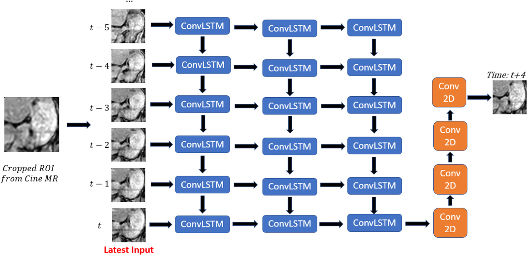
Figure 2. ConvLSTM network structure. Blue blocks represent convLSTM layer, and orange blocks represent convolution 2D layer.
Download figure:
Standard image High-resolution image2.3. Data pre-processing
Prior to inputting the data into the network, several pre-processing steps were performed on the cine images. First, all the cine images were resized to a dimension of 352 by 352, and specific regions of interest (ROIs) were cropped, with a separate ROI for each organ of interest. The selected ROIs included the stomach, liver, kidney, and pancreas. Coronal images were chosen for the stomach and liver, while axial images were selected for the kidney and pancreas. Detailed information regarding the ROIs is provided in table 2. It is important to note that the visibility and identification of certain organs varied across datasets, resulting in different numbers of datasets available for each ROI, as indicated in the last column of the table. For example, the pancreas is only available in 5 out of the 17 datasets.
Table 2. Description of the ROIs cropped from cine-MR images included in the study. The images were resized to 352 by 352 before ROI cropping in order to preserve the magnitude between different datasets.
| ROI | Size | Orientation | Number of datasets |
|---|---|---|---|
| Stomach | 80 × 80 | Coronal | 14 |
| Liver | 160 × 160 | Coronal | 16 |
| Pancreas | 120 × 60 | Axial | 5 |
| Kidney | 80 × 80 | Axial | 16 |
| Total | Multiple | 17 |
After cropping the images, additional pre-processing steps were performed to enhance image quality, including contrast adjustment, median filtering, and other de-noising techniques. Subsequently, the dataset underwent data partitioning ,as depicted in figure 3, where the images were divided into training, validation, and test datasets using a fixed ratio of 8:1:2, respectively. This consistent partition ratio was employed across different datasets to ensure comparability in subsequent analyzes and evaluations. The images are further partitioned into input images, prediction frames, and output image in training data, validation data, and test data. Input images are used to generate the predicted output image. The predicted output image is then compared with the ground truth output image, as well as the last frame of input images, which is referred as image without prediction in the following text.

Figure 3. (a) Describes the partition of training data, validation data, and test data of the whole dataset, and (b) describes the partition of input images, prediction frames, and output image(s) in training data, validation data, and test data. The predicted output image is compared with the ground truth output image, as well as the last frame of input images, which is referred as image without prediction in the following description. Note that the time interval (0.6 s), as well as the number of input frames, predictions frames, and output frame are just for demonstration. The actual number may be different for each dataset.
Download figure:
Standard image High-resolution image2.4. Model training
The convLSTM model was implemented, trained, and evaluated using the Tensorflow 2.6.0 framework and the Adam optimizer in a Python 3.9.7 environment. The training process utilized an NVidia A100 GPU with 80 GB memory and an AMD EPYC 7742 64-Core CPU for computational tasks.
Prior to the individual training phase, a hyperparameter selection process was conducted on the Stomach dataset 2–3 for coronal images and Kidney dataset 2–3 for axial images. This dataset was chosen because the stomach in this dataset exhibits a more complex motion behavior compared to other datasets, and the kidney boundaries in the dataset are distinctly delineated.
Multiple hyperparameters were fine-tuned to determine the optimal configuration of the model, including the number of convolution filters, dropout rate, number of epochs, choice of loss function, kernel size, and input size. During the tuning process, each hyperparameter was adjusted while maintaining the other hyperparameters constant to ensure controlled experimentation. The initial hyperparameter setup consisted of 64 convolutional filters with a filter kernel size of 3 by 3 for each of the three convLSTM layers, the SSIM loss function, 30 epochs, 4 frames as prediction interval, 6 input frames, and 0 dropout rate. Once the optimal hyperparameters were determined, the resulting model was referred to as the Optimal Model and was subsequently applied to other datasets through individual training and transfer learning approaches.
In individual training, the training, validation, and test data were sourced from the same dataset. In transfer learning, 10 datasets were used for training and validation, while the remaining 6 datasets were employed for fine-tuning and testing. Transfer learning techniques were employed to transfer the globally trained model to the specific test sets. Therefore, the test set was completely unseen by the model if fine-tuning was not used. However, the model can be fine-tuned when being applied to the new dataset. Due to limitations in the available datasets, only the kidney and liver went through transfer learning phase. Each case was trained five times, and the average performance was calculated.
It's crucial to clarify that the term 'Optimal Model' does not mean the model is universally optimal across all datasets or organs. Separate Optimal Models were chosen for coronal and axial images, recognizing that a model excelling with coronal images might not perform as well for axial ones. The choice of optimal hyperparameter set is influenced by numerous factors, with the primary goal being consistent and reasonable outputs across diverse datasets. This paper does not delve into optimal hyperparameters for each individual dataset.
The details of hyperparameters that we have examined are listed below:
2.4.1. Prediction interval
The number of prediction frames indicates the interval of time that the model attempts to predict. For example, in Dataset 2–3, where the time interval between two frames is 0.58 s, a prediction frame length of 4 frames corresponds to a total prediction time interval of 2.32 s, which is approximately half of the usual human's breathing cycle. The largest motion-error due to respiration may occur at around this time offset as shown in figure 6. In this study, we have tested intervals ranging from 1 to 50 frames. Interval length of 4 frames was used as default when other hyper-parameters were being tested because it represents the most challenging time interval.

Figure 4. Boxplot of the Performance of all hyperparameters examined for the optimal model for coronal images. (a) number of convolution filters, (b) input number, (c) loss function, (d) other hyperparameters. At the x-axis, the box with solid line refers to the default set up, the box with dashed line refers to the selected set up. Here all selected hyperparameters were default hyperparameters, so solid line and dash line both refer to the same hyperparameter.
Download figure:
Standard image High-resolution image2.4.2. Loss functions
Various loss functions were employed for comparison, including SSIM, mean square error (MSE), and mean absolute error (MAE). SSIM was used as default.
SSIM is an image comparison metric commonly used to assess the similarity between two images. The SSIM formula is defined as follows:


where μx and μy are the mean intensity, σx and σy are the standard deviation estimation of the images, σxy is the covariance between image x and image y , K1 and K2 are 0.01 and 0.03, respectively, based on the standard implementation (Wang et al 2004). L is the dynamic range of the pixel values. In actual usages, the SSIM of images are calculated based on the mean SSIM value of various windows of an image, with the default window size 11 by 11.
MSE is defined as

where xi and yi are the pixel grayscale intensity values of corresponding pixels with index i. MAE, similar to MSE, is defined as

2.4.3. Number of input frames
The length of the input data is determined by the number of input frames. We conducted experiments using 5, 6, 7, 8, 9, and 10 input frames. The length of 6 was used as default for input.
2.4.4. Number of epochs
The number of epochs defines the number of times the training dataset is iterated during the training process. Selecting an appropriate number of epochs is crucial to ensure complete training without overfitting. Insufficient epochs may result in incomplete training, while excessive epochs may lead to wasted time and increased risk of overfitting. The epoch number of 30 (default) and 40 were tested.
2.4.5. Dropout
Dropout is a regularization technique used to prevent overfitting in neural networks. It involves randomly dropping out a certain percentage of nodes during training. In the convLSTM network, there are two types of dropout: conventional dropout, which controls the fraction of units dropped for the linear transformation of inputs, and recurrent dropout, which controls the fraction of units dropped for the linear transformation in the temporal direction. Two models with a dropout rate of 0.1 in either inputs or recurrent states were used to compare with the default model which is without dropout.
2.4.6. Convolution filters
The number of convolution filters determines how many filters exist at each layer of the convLSTM network. We utilized a three-layer convLSTM architecture and tested different combinations of convolution filters, including (32, 32, 32), (64, 64, 64), (96, 96, 96), (32, 32, 64), (32, 64, 32), (32, 64, 64), (32, 64, 96), (64, 32, 32), (64, 32, 64), (64, 64, 32), and (96, 64, 32). The default set up was (64, 64, 64), which refers that there are 64 convolutional filters for each of the three layers in convLSTM network.
2.4.7. Kernel size
The kernel size in convolutional layers determines the 2D convolutional window used on the image in each filter in the network. We conducted experiments using kernel sizes of 3 by 3 (default) and 5 by 5.
2.5. Individual training on different organs
After obtaining the optimal model, we applied it to each dataset for comparison. The ROIs included stomach, kidney, pancreas, and liver. The data partition method was mentioned in 2.3. The output images were saved for comparison with ground truth.
2.6. Transfer learning
Transfer learning is based on the idea that if a model is trained on a large and comprehensive dataset, then it can effectively learn general features that can be applicable to other tasks. Instead of starting from scratch, transfer learning typically uses a a model pre-trained on a large dataset and then apply it to a new and smaller dataset, with or without fine-tuning. Transfer learning allows for leveraging pre-existing models, reducing both computational cost and training time. Also, it often leads to improved performance, especially in tasks where the available dataset is relatively small.
Transfer learning was implemented for the liver and kidney datasets. We used 10 datasets for initial training and validation, while the remaining 6 datasets were dedicated to testing and fine-tuning. For each training dataset, approximately  of the data were used as the training set for transfer learning, and the remaining portion served as the validation set. This resulted in a total of 8284 training images and 1036 validation images. After the training process was finished, the trained model was then applied to test set via transfer learning. Regarding the test set, approximately
  of the data were utilized for fine-tuning of transfer learning,
  for validation, and the last
  for final testing. The final test set was used as the sole test set regardless of whether fine-tuning was involved or not.
2.7. Evaluation metrics
To assess the performance of image prediction, we utilized several image comparison metrics. The metrics employed in our experiments include structural similarity index (SSIM), normalized root mean square error (NRMSE), NCC, and PSNR.
NRMSE is a normalized variant of MSE ranged from 0 to 1 for better visualization.  is the average intensity of the reference image. NRMSE and related normalized mean square error (RMSE) are defined as:


NCC is a normalized index measuring correlation between two variables. The 2D NCC is defined as

where NCC is normalized correlation coefficient between two 2D variables x and y, m and n are the row and the column indices, respectively,  and
and  are the average value of x and y.
PSNR is defined as

where MAXI is the maximum possible pixel value of the image, typically 65 535 for 16 bit images.
3. Results
3.1. Optimal model
Boxplot figures 4 and 5 show the prediction performances with various hyperparameters in order to find the optimal hyperparameter combinations for both coronal and axial image datasets. The boxes in boxplot display results based on the five-number summary: the maximum value, the 75% quartile, the sample median, the 25% quartile and the minimum value. The comparison metric used for selection is SSIM score. If one hyperparameter variation showed a higher score than the default setup and also showed a statistically significant difference, then the hyperparameter was selected instead of the default parameter. The statistical significance was calculated based on p-value with an alpha of 0.05 signifying a significant difference which was obtained by comparing the SSIM score of the test model with the default model. For coronal images, all hyperparameters in the default setup were selected for the optimal model. For axial images, the optimal model was selected with loss function of MAE, input number of 6, and the number of convolution filters of 96, 96, and 96.

Figure 5. Boxplot of the performance of all hyperparameters examined for the optimal model for axial images. (a) number of convolution filters, (b) input number, (c) loss function, (d) other hyperparameters. A the x-axis, the box with solid line refers to the default set up, the box with dashed line refers to the selected set up.
Download figure:
Standard image High-resolution imageFigure 6 displays prediction results based on varying time intervals while maintaining other hyperparameters consistent with the optimal model. As time intervals increase, the SSIM score of prediction starts to steadily and slowly drop. In the default model, four frames which roughly equate to 2.4 s in most datasets was used as time interval. It is about half of the human breath cycle time, which represents the largest motion offset due to respiration. In order to prove the model's proficiency in predicting a challenging period of time, an interval of four frames was utilized as time interval in subsequent experiments. Figure 7 offers a visual comparison of the ground truth image (first row), predicted image (second row), and the image without any prediction (third row), as well as their pixel intensity disparities with the ground truth for stomach, liver, kidney, and pancreas. This predicted representation indicates motion projected 2.4 s ahead from the most recent input. The pixel-wise difference between the ground truth and the prediction is noticeably smaller than the difference between the ground truth and the latest input for all ROIs.

Figure 6. (a)–(d) shows how the prediction SSIM score changes as time interval increases for stomach, liver, kidney, and pancreas dataset. Blue dots show the SSIM score performance of the optimal model, and orange dots show the SSIM scores for the images without prediction.
Download figure:
Standard image High-resolution image3.2. Model performance in different organs, individual training
The model performance was also displayed quantitatively using different metrics besides visual comparison. Tables 3–6 show the model performance scores in stomach, liver, kidney, and pancreas. Despite variations across datasets and organs, our predictions generally enhance the image similarity across most metrics, with only a few exceptions. The average SSIM scores for stomach, liver, kidney, and pancreas are 0.538, 0.641, 0.772, and 0.661, respectively.
Table 3. Prediction model performance of stomach area (individual training).
| Prediction | No Prediction | |||||||
|---|---|---|---|---|---|---|---|---|
| Dataset | SSIM | NRMSE | NCC | PSNR | SSIM | NRMSE | NCC | PSNR |
| 1–2 | 0.540 | 0.374 | 0.770 | 16.920 | 0.419 | 0.457 | 0.650 | 15.312 |
| 1–3 | 0.594 | 0.263 | 0.840 | 18.246 | 0.333 | 0.433 | 0.530 | 14.215 |
| 1–4 | 0.378 | 0.390 | 0.618 | 13.394 | 0.229 | 0.463 | 0.385 | 11.924 |
| 1–5 | 0.632 | 0.291 | 0.827 | 19.184 | 0.511 | 0.374 | 0.734 | 17.092 |
| 1–6 | 0.604 | 0.222 | 0.880 | 18.553 | 0.366 | 0.314 | 0.747 | 15.544 |
| 1–7 | 0.443 | 0.305 | 0.787 | 15.375 | 0.401 | 0.310 | 0.730 | 15.373 |
| 2–1 | 0.539 | 0.287 | 0.797 | 16.338 | 0.302 | 0.347 | 0.568 | 14.649 |
| 2–2 | 0.558 | 0.219 | 0.902 | 19.962 | 0.368 | 0.312 | 0.801 | 16.957 |
| 2–3 | 0.530 | 0.246 | 0.853 | 17.339 | 0.308 | 0.348 | 0.672 | 14.393 |
| 2–4 | 0.418 | 0.393 | 0.660 | 15.020 | 0.258 | 0.486 | 0.456 | 13.301 |
| 2–5 | 0.548 | 0.338 | 0.717 | 18.003 | 0.405 | 0.393 | 0.499 | 16.798 |
| 2–6 | 0.574 | 0.234 | 0.875 | 18.569 | 0.432 | 0.288 | 0.780 | 17.083 |
| 2–7 | 0.579 | 0.201 | 0.891 | 18.438 | 0.376 | 0.276 | 0.759 | 15.736 |
| 2–8 | 0.593 | 0.367 | 0.830 | 19.959 | 0.423 | 0.476 | 0.664 | 18.002 |
Table 4. Prediction model performance of liver area (individual training).
| Prediction | No Prediction | |||||||
|---|---|---|---|---|---|---|---|---|
| Dataset | SSIM | NRMSE | NCC | PSNR | SSIM | NRMSE | NCC | PSNR |
| 1–1 | 0.685 | 0.226 | 0.889 | 18.535 | 0.668 | 0.167 | 0.864 | 20.931 |
| 1–2 | 0.718 | 0.215 | 0.885 | 20.375 | 0.598 | 0.254 | 0.810 | 19.091 |
| 1–3 | 0.684 | 0.218 | 0.857 | 19.646 | 0.435 | 0.329 | 0.665 | 16.138 |
| 1–4 | 0.595 | 0.298 | 0.786 | 17.403 | 0.451 | 0.376 | 0.638 | 15.472 |
| 1–5 | 0.746 | 0.159 | 0.948 | 22.235 | 0.633 | 0.188 | 0.917 | 20.918 |
| 1–6 | 0.642 | 0.380 | 0.885 | 18.483 | 0.456 | 0.427 | 0.765 | 17.534 |
| 1–7 | 0.629 | 0.268 | 0.816 | 16.391 | 0.560 | 0.249 | 0.771 | 17.296 |
| 2–1 | 0.663 | 0.199 | 0.897 | 19.262 | 0.453 | 0.255 | 0.779 | 17.303 |
| 2–2 | 0.586 | 0.251 | 0.890 | 19.775 | 0.416 | 0.333 | 0.786 | 17.443 |
| 2–3 | 0.623 | 0.229 | 0.915 | 19.733 | 0.376 | 0.302 | 0.799 | 17.499 |
| 2–4 | 0.573 | 0.276 | 0.836 | 18.351 | 0.397 | 0.360 | 0.703 | 16.223 |
| 2–5 | 0.587 | 0.207 | 0.813 | 18.075 | 0.419 | 0.274 | 0.643 | 15.777 |
| 2–6 | 0.585 | 0.273 | 0.824 | 16.846 | 0.449 | 0.278 | 0.692 | 17.118 |
| 2–7 | 0.639 | 0.216 | 0.875 | 18.054 | 0.392 | 0.267 | 0.711 | 16.346 |
| 2–8 | 0.655 | 0.234 | 0.842 | 18.950 | 0.482 | 0.334 | 0.668 | 16.174 |
Table 5. Prediction model performance of kidney area (individual training).
| Prediction | No Prediction | |||||||
|---|---|---|---|---|---|---|---|---|
| Dataset | SSIM | NRMSE | NCC | PSNR | SSIM | NRMSE | NCC | PSNR |
| 1–1 | 0.829 | 0.134 | 0.968 | 23.733 | 0.822 | 0.120 | 0.965 | 24.675 |
| 1–2 | 0.735 | 0.301 | 0.857 | 17.426 | 0.678 | 0.374 | 0.786 | 15.942 |
| 1–3 | 0.768 | 0.165 | 0.950 | 20.898 | 0.627 | 0.264 | 0.864 | 16.961 |
| 1–4 | 0.845 | 0.161 | 0.945 | 21.197 | 0.741 | 0.232 | 0.885 | 18.156 |
| 1–5 | 0.772 | 0.168 | 0.946 | 21.965 | 0.679 | 0.224 | 0.908 | 19.512 |
| 1–6 | 0.811 | 0.195 | 0.945 | 20.878 | 0.621 | 0.339 | 0.845 | 15.864 |
| 1–7 | 0.736 | 0.267 | 0.875 | 18.533 | 0.704 | 0.309 | 0.825 | 17.586 |
| 2–1 | 0.806 | 0.143 | 0.968 | 23.083 | 0.667 | 0.244 | 0.910 | 18.493 |
| 2–2 | 0.746 | 0.213 | 0.932 | 20.153 | 0.626 | 0.315 | 0.861 | 16.791 |
| 2–3 | 0.751 | 0.216 | 0.933 | 20.305 | 0.556 | 0.375 | 0.802 | 15.560 |
| 2–4 | 0.681 | 0.264 | 0.871 | 17.875 | 0.546 | 0.363 | 0.765 | 15.160 |
| 2–5 | 0.843 | 0.124 | 0.961 | 27.493 | 0.733 | 0.192 | 0.915 | 23.709 |
| 2–6 | 0.757 | 0.194 | 0.943 | 20.836 | 0.637 | 0.265 | 0.878 | 18.277 |
| 2–7 | 0.725 | 0.234 | 0.913 | 18.976 | 0.529 | 0.403 | 0.754 | 14.610 |
| 2–8 | 0.772 | 0.161 | 0.950 | 23.257 | 0.649 | 0.247 | 0.884 | 19.769 |
Table 6. Prediction model performance of pancreas area (individual training)
| Prediction | No Prediction | |||||||
|---|---|---|---|---|---|---|---|---|
| Dataset | SSIM | NRMSE | NCC | PSNR | SSIM | NRMSE | NCC | PSNR |
| 1–6 | 0.669 | 0.267 | 0.845 | 17.596 | 0.506 | 0.377 | 0.704 | 14.632 |
| 2–1 | 0.716 | 0.168 | 0.926 | 21.191 | 0.526 | 0.271 | 0.812 | 17.170 |
| 2–3 | 0.638 | 0.231 | 0.889 | 18.728 | 0.440 | 0.362 | 0.739 | 14.918 |
| 2–5 | 0.619 | 0.212 | 0.859 | 18.958 | 0.453 | 0.288 | 0.738 | 16.432 |
| 2–7 | 0.664 | 0.207 | 0.877 | 18.866 | 0.504 | 0.305 | 0.733 | 15.708 |
3.3. Transfer learning
Table 7 and table 8 present the prediction results for the kidney and liver datasets using transfer learning. The tables are divided into three sections: the first section shows the prediction results with fine-tuning, the second section shows the performance without fine-tuning, and the last section displays the image similarity without prediction.
Table 7. Prediction model performance of kidney area (transfer learning).
| Transfer learning | Fine-tuning | No fine-tuning | No prediction | |||
|---|---|---|---|---|---|---|
| Dataset | SSIM | NRMSE | SSIM | NRMSE | SSIM | NRMSE |
| 1–1 | 0.829 | 0.140 | 0.479 | 0.461 | 0.813 | 0.128 |
| 1–2 | 0.713 | 0.336 | 0.390 | 0.673 | 0.676 | 0.376 |
| 1–3 | 0.764 | 0.178 | 0.406 | 0.645 | 0.628 | 0.263 |
| 1–4 | 0.830 | 0.185 | 0.232 | 0.757 | 0.741 | 0.232 |
| 1–5 | 0.780 | 0.164 | 0.715 | 0.196 | 0.680 | 0.223 |
| 3–2 | 0.735 | 0.317 | 0.401 | 0.600 | 0.515 | 0.461 |
Table 8. Prediction model performance of liver area (transfer learning).
| Transfer learning | Fine-tuning | No fine-tuning | No prediction | |||
|---|---|---|---|---|---|---|
| Dataset | SSIM | NRMSE | SSIM | NRMSE | SSIM | NRMSE |
| 1–1 | 0.693 | 0.217 | 0.623 | 0.218 | 0.668 | 0.167 |
| 1–2 | 0.725 | 0.213 | 0.712 | 0.236 | 0.598 | 0.254 |
| 1–3 | 0.682 | 0.219 | 0.596 | 0.258 | 0.435 | 0.329 |
| 1–4 | 0.599 | 0.309 | 0.594 | 0.307 | 0.451 | 0.376 |
| 1–5 | 0.756 | 0.164 | 0.683 | 0.186 | 0.633 | 0.188 |
| 3–1 | 0.707 | 0.244 | 0.628 | 0.333 | 0.518 | 0.348 |
3.4. Computation time
The total computation time of model inference is much smaller than current latency time in MR-Linac The computation time to generate one predicted image for smaller ROIs like stomach is less than 10ms, and the computation time for larger ROIs (liver) is around 100ms, given single GPU.
4. Discussion
4.1. Hyperparameter selection
4.1.1. Input image frames
Figure 4 and figure 5 illustrate that for a prediction time interval of 4 frames, the input number of 6 results in the best average SSIM performance for coronal images and the input frames of 10 works best for axial images. This finding suggests that for different organs with different orientations, the number of inputs that is needed to provide sufficient information for accurate motion prediction may be different. The optimal input image frames may be related to the breathing cycle which is about 8–10 frames in this case. For coronal images, in order to predict one image 4 frames ahead, an input number of 6 is more likely to capture the corresponding breathing state of ROI of the object image from the previous breathing cycle, compared to an input number of 5, which sometimes may fail to cover a full breathing cycle. For axial images, the number of inputs for optimal outcome is 10, which is around a full breathing cycle. The difference of the optimal input frames may due to the fact that the motion of ROIs is largely superior–inferior.

Figure 7. Prediction result comparison of different organs between ground truth, predicted image, and image without prediction. For each organ ROI, the first column shows the image, and the second column shows the pixel-wise intensity difference with the ground truth image.
Download figure:
Standard image High-resolution image4.1.2. Convolutional filters
Multiple numerical combinations of convolutional filters were compared to the default model for coronal images, but only slight differences in prediction SSIM scores were observed. These differences were not significant enough to justify selecting an alternative combination. On the other hand, a larger number of convolution filters did increase the prediction performance for axial images. It indicates that the optimal number of extracted features for motion prediction is different with different views. Again, the reason could be that most of the motion was captured in coronal view while not captured in axial view.
4.1.3. The choice of loss function
Three loss functions (SSIM, MSE, and MAE) were compared to find the one with the optimal performance. It was not surprising that SSIM loss function exhibited the highest SSIM score for coronal images. However, MAE loss function exhibits an even higher score than SSIM loss function for axial images. On the other hand, MSE exhibited a significantly lower performance compared to the other loss functions for both coronal images and axial images. This disparity may be attributed to the fact that MSE is more sensitive to outliers compared to the other loss functions due to its squaring part.
4.1.4. Dropout
Conventional dropout had a more pronounced influence compared to recurrent dropout. However, overfitting was unlikely to have occurred in our experiment, indicating that dropout was not necessary.
4.1.5. Other hyperparameters
The choice of kernel size in the convolution computation of the network was investigated. While larger kernels are typically suited for faster motion and smaller kernels for slower motion, no significant improvement was found between 3 by 3 and 5 by 5 kernels, leading to the retention of the original kernel size. Additionally, increasing the number of epochs did not impact the model's performance, suggesting that the loss function had already reached its minimum within 30 epochs.
4.2. Prediction time intervals
Figure 6 demonstrates the effect of increasing prediction time interval on performance. It is evident that the model achieves the highest SSIM score when the interval is 1 frame. However, even at larger intervals, beyond approximately 10 frames, the prediction SSIM scores stabilize. Although the scores for these larger intervals are not as high as those for smaller intervals, they still exhibit a higher similarity with the ground truth compared to the corresponding image without prediction. Notably, a discernible pattern is observed in the SSIM score without prediction, indicating the presence of periodic motion in the organs. This pattern is also evident in the liver, pancreas, and kidney datasets (figures 6(b)–(d)), which has a period about 10 frames or 6 s, likely mainly contributed by respiration cycle. The similarity score is higher when the prediction interval time aligns with respiration, while it decreases when the prediction interval time corresponds to the opposite phase of respiration.
4.3. Organ specific prediction
Different organs display varying prediction performances, with the kidney generally exhibiting better performance than the liver. Several factors, such as image pixel size, image orientation, and organ motion patterns, could contribute to this disparity in prediction accuracy. Nevertheless, the SSIM score without prediction curve demonstrates a similar pattern across all four organs (figure 6). This suggests that all four organs are at least partially affected by a common type of motion, likely respiratory motion, as indicated by the peak values around frames 9 and 19.
The SSIM score in our study was relatively lower compared with some studies using PCA and other methods. For example, recently, results from a PCA modelling paper using 4DCT achieved SSIM of 0.88 for chest region (Asano et al 2023). For comparison, our SSIM values were 0.5–0.6. However, it is important to note that the PCA result was based on whole uncropped 4DCT chest images, which included mostly stationary anatomy. Our SSIM is based on a cropped ROI which includes mostly moving anatomy, so our lower SSIM values are to be expected. Most importantly, the LSTM model results are for predicted images for future target position rather than current position. As well, the PCA model deals with simpler target motion pattern in lung compared to abdominal motion which is more complex.
4.4. Robustness
To assess the robustness of the model, we evaluated the SSIM scores for all images in the test set (figure 8). The robustness of a test set is defined as the ratio of effective predictions (prediction SSIM score higher than the score without prediction) to the total number of images in the test set. The robustness scores for all test sets are presented in table 9. Notably, the stomach test set achieved a robustness of 79.75%, indicating that the model was effective for around 80% of the images in the stomach dataset. Moreover, one liver dataset used in transfer learning achieved a robustness score of one, indicating that the prediction model successfully improved the image similarity for all images in this dataset. The overall average test set robustness was 82.1%.

Figure 8. SSIM score among all the images in one stomach test set, the robustness is 0.885.
Download figure:
Standard image High-resolution image
Table 9. Robustness of all the test sets. liver transfer learning and kidney transfer learning refer to the test set used in transfer learning phase.
| Test set | Stomach | Liver | Kidney | Pancreas | Liver transfer learning | Kidney transfer learning | Average |
|---|---|---|---|---|---|---|---|
| Robustness | 0.797 | 0.806 | 0.810 | 0.891 | 0.829 | 0.791 | 0.821 |
4.5. Transfer learning
Table 7 and table 8 compare the prediction results for kidney and liver datasets using transfer learning. The tables are divided into three sections: performance with fine-tuning, performance without fine-tuning, and image similarity without prediction. It can be observed that transfer learning with fine-tuning has a beneficial impact on prediction accuracy. The SSIM scores are consistently higher when fine-tuning is applied compared to the case without prediction, especially in table 7. While the transfer learning model performs relatively poorly in some datasets without fine-tuning, the application of fine-tuning largely compensates for the performance difference.
4.6. Future work
A primary issue is that our current model necessitates cropping the region of interest (ROI) from cine-MR images. Using full-size images without this cropping results in diminished performance in organ motion tracking. Another limitation is that our model only processes one plane from a three-planar dataset, thereby ignoring potential insights from the remaining planes. Furthermore, the 2D model's intrinsic constraint is its inability to monitor organ motion beyond its current plane. To address these drawbacks, we're in the process of designing a 3D cine-MR motion prediction algorithm, which would allow motion tracking in all three dimensions. Although 3D cine-MR is still not a mature technique and is faced with multiple issues, some promising results have been published (Wu et al 2023). This 3D model development is our imminent research focus.
5. Conclusion
In our study, we introduced a straightforward 2D cine-MR prediction algorithm tailored for MR-Linac radiotherapy. The cine-MR dataset, comprising 17 sets from MR-sim, mirrored the Unity sequence in MR-Linac These datasets, spanning duration from 1 to 10.6 min, were processed, cropped, and categorized into stomach, liver, kidney, and pancreas groups.
We formulated a convLSTM model adept at forecasting multiple abdominal organs via MR-sim for a prediction time interval that has the maximal offset from intra-cycle motion. Our model is able to compute a prediction image at a future time with a computation time that is significantly less than prediction interval. By judiciously selecting hyperparameters, we maximized the model's performance. We have also implemented the model with individual training, transfer learning with and without fine-tuning. Our findings highlighted enhanced image similarity for predicted images compared to non-predicted ones, underscoring our method's potential in reducing lag between real-time image capture and beam delivery in MR-Linac radiotherapy. Looking ahead, our aim is to surmount the existing model's limitations and design a 3D cine MR motion prediction framework.
Acknowledgments
We would like to thank Dr Walter O'Dell (University of Florida) for his helpful comments during preparation of this manuscript; and Drs Kaleb Smith and Huiwen Ju (NVIDIA Corporation) for their programming suggestions. We also want to thank the University of Florida Research Computing for generously providing computing resources on the HiPerGator cluster.
Data availability statement
The data cannot be made publicly available upon publication because no suitable repository exists for hosting data in this field of study. The data that support the findings of this study are available upon reasonable request from the authors.
Ethical statement
This study was approved by the Institutional Review Board (IRB) of the University of Florida IRB202301309. All procedures were carried out in accordance with the ethical rules and the principles of the Declaration of Helsinki. The need for informed consent was waived by IRB because the study was retrospective.