
Abstract
The major part of energy deposition of ionizing radiation is caused by secondary electrons, independent of the primary radiation type. However, their spatial concentration and their spectral properties strongly depend on the primary radiation type and finally determine the pattern of molecular damage e.g. to biological targets as the DNA, and thus the final effect of the radiation exposure. To describe the physical and to predict the biological consequences of charged ion irradiation, amorphous track structure approaches have proven to be pragmatic and helpful. There, the local dose deposition in the ion track is equated by considering the emission and slowing down of the secondary electrons from the primary particle track. In the present work we exploit the model of Kiefer and Straaten and derive the spectral composition of secondary electrons as function of the distance to the track center. The spectral composition indicates differences to spectra of low linear energy transfer (LET) photon radiation, which we confirm by a comparison with Monte Carlo studies. We demonstrate that the amorphous track structure approach provides a simple tool for evaluating the spectral electron properties within the track structure. Predictions of the LET of electrons across the track structure as well as the electronic dose build-up effect are derived. Implications for biological effects and corresponding predicting models based on amorphous track structure are discussed.
Export citation and abstract BibTeX RIS

Original content from this work may be used under the terms of the Creative Commons Attribution 4.0 licence. Any further distribution of this work must maintain attribution to the author(s) and the title of the work, journal citation and DOI.
1. Introduction
The DNA damage pattern and biological consequences of ionizing radiation are well known to depend not only on biological factors (e.g. cell type, cell cycle and radiosensitivity) but also on the type of radiation. This is well established and accounted for within the concept of radiation weighting factors in radiation protection or the concept of relative biological effectiveness (RBE) in radiation biology and particle therapy. While different radiation types such as orthovoltage x-rays or ions with high linear energy transfer (LET) differ in the nanoscopic and microscopic energy distribution within the target, notably in both cases most of the energy is transferred to the target material via secondary electrons, causing higher order electron generations in cascades of further ionisations.
In the case of photon radiation, secondary electrons are produced in an energy dependent manner via Compton ionization or the photoelectric effect (at photon energies relevant in radiation therapy). For very low energies of the order of a few keV or less, so called ultrasoft x-rays (Goodhead and Nikjoo 1989), practically only the latter plays a role. In this process the energy of the photon is transferred to the photoelectron, which dispenses its kinetic energy in several further ionisations and excitations spread over some nanometres. A clustered ionization pattern is established, which potentially causes complex DNA damage. In that context the relevance of low-energetic secondary electrons, so-called track-ends, has been extensively studied both experimentally and theoretically (Nikjoo and Lindborg 2010). It was found that the spatial clustering of ionisations towards the end of electron tracks is more effective per deposited energy unit than ionisations along the higher energetic portion of electron tracks.
Concerning ion radiation, secondary and higher generation electrons lead to a track structure of energy deposition around the ion's trajectory. As secondary electrons are emitted based on a ballistic scattering process, such emission is associated with an angle and related energy distribution. Typically a broad energy spectrum of secondary electron establishes, where the low energies occur more frequent than higher ones. Depending on the radial position within the track structure the spectrum will vary due to the energy dependent range of electrons. This ultimately leads to the well known decrease of dose with increasing distance to the track center (Kiefer and Straaten 1986), but also to a variation of the biological effectiveness (Cucinotta et al 1999) across the track.
Secondary electrons are often called δ-electrons. Usually this term is used for all liberated electrons along their track, while in the present work we mostly mean the first generation of liberated electrons which give rise to track structure formation, whose initial kinetic energy, however, also contains the energy transmitted to further generation secondary electrons.
A theoretic approach to capture the main properties of δ-ray emission from the particle trajectory was to take into account the cross section of δ-electron production. In an early approach by Butts and Katz (1967) electrons were assumed to propagate perpendicular outward from the track center. A more detailed implementation of collision dynamics carried out by Kiefer and Straaten (1986) led to considering the double differential cross section, i.e. an energy-dependent emission angle of δ-rays. In this document we follow this theoretic framework describing the formation and transport of δ-electrons emerging from ion tracks.
Amorphous track structure representations are used in biophysical models aiming to predict ion effects based on the local dose deposition. This notion exploits the definition of dose as the absorbed energy per mass in the limit of small volumes, therefore being a point quantity. The Katz model (Butts and Katz 1967) actually stimulated the derivation of an amorphous track structure expression from Bohr's atom theory. The Local effect model, which is used for treatment planning in carbon ion centres in Europe, uses the improved track structure formulation by Kiefer and Straaten (1986). Microdosimetric approaches such as the microdosimetric kinetic model originally start off from microdosimetric spectra without an explicit need for amorphous track structure models. However, pragmatic implementations employ the track structure model of Kiefer and Chatterjee to derive all necessary information, and such implementations are used used to assess the RBE gradient in treatment planning in Japanese carbon ion facilities (Kase et al 2008, Inaniwa et al 2010). An overview of different amorphous track structure models including a discussion of their experimental and theoretic limitations is given in (Elsässer et al 2008).
In radiobiological effect models, the inflicted DNA damage is assumed to be in proportion to the local energy concentration, often also termed local dose or in the framework of microdosimetry the expectation value of the specific energy. In that spirit all three mentioned models make use of the amorphous track structure to predict the damage yield after high-LET irradiation based on the yields for low-LET radiation. However, the spectral composition of secondary electrons in an ion's track structure may differ from the one in a low-LET radiation field such as orthovoltage x-rays. In particular, the relative contribution by track ends is expected to be higher especially in the center and at the ridges of the ion track. The models therefore conceptually underestimate the DNA damage yield in these regions. A simple improvement of this flaw is to include the effectiveness of secondary electrons with respect to DNA damage induction and by appropriate weighting calculate the yield of the considered spectral electron mixture. Integrating over ion tracks one can finally determine DNA yields, which depend on the local dose pattern but now as well on the spectral composition therein. In the recent development stage of the Local effect model, LEM IV, the underestimate of the RBE in the entrance channel was often attributed to neglecting the enhanced effectiveness of the secondary electrons (Pfuhl et al 2022a, 2022b). Typically a higher fraction of low energetic, more effective secondary electrons in ion tracks as compared to photon reference radiation results in an increase of radiation induced DNA damage.
The purpose of this work is to inspect the variation of radiation quality across the track structure of individual ions. In that respect, we use the term 'radiation quality' as representative for the spectral composition of secondary electrons and the associated energy loss. The results are compared to Monte Carlo calculations. With the here presented approach an estimate of the effectiveness of secondary electrons across the particle track becomes feasible and paves the way to fully include the electron's efficacy in the ultimate effect calculations of the ions. A corresponding development is on the way.
2. Methods
2.1. The Kiefer–Straaten track structure model
2.1.1. Secondary electron production
By means of ion-atom collision processes, the number dN of δ-electrons produced in the kinetic energy interval dT0 per length segment dz along the ion path is given by

where Z* is the effective charge of the ions passing through matter according to the empirical Barkas formula

and β is the relativistic velocity parameter characterizing the ion speed. The prefactor equates to C = 8.5 eV μm−1 for liquid water. This result is obtained from the classical (non quantum mechanical) derivation of the Bethe equation describing the energy loss of heavy charged particles in matter, which goes back to Bohr (1915). In this formalism the electron number density in the target material and the momentum transfer to any electron at distance b (impact parameter) to the ion trajectory are considered. If for the latter the relativistic energy–momentum relation is used, equation (1) is modified as

where me labels the electron rest mass and c the speed of light in vacuum. Note that albeit this relativistic correction the approach to equate the kinetic energy transfer to secondary electrons is still classical. A full derivation of equation (3) is given in appendix A. Notably the production cross section expressed by equations (1) and (3) only contains Z*2 as a scaling factor, while the shape of the spectrum does not depend on the ion type but only on the energy. Hence, at a given ion energy the kinetic energy spectrum of secondary electrons is the same for all ion types at a given energy.
2.1.2. Scattering kinematics
The kinetic energy transferred to the electron is linked to an emission angle θ via

Therein, the maximum transferable energy derives from knock-on collisions as

with M as the rest mass of the ion and the relativistic factor  . As me
≪ M the approximation is usually valid except for ultrarelativistic cases (Workman et al
2022). A derivation of equations (4) and (5) is given in appendix B.
. As me
≪ M the approximation is usually valid except for ultrarelativistic cases (Workman et al
2022). A derivation of equations (4) and (5) is given in appendix B.
2.1.3. Secondary electron range and dose deposition
The range of the δ-electrons at kinetic energy T can be parameterized empirically as

where the scaling constants for liquid water are K = 4.18 × 10⁻¹¹ cm eV−α and α = 1.7, see Kiefer and Straaten (1986). This range is the projected range and not the entire path length the electron travels until it stops or gets absorbed. Equations (3)–(6) are the basic equations of the track structure model which allow to calculate the electron spectrum and the associated energy loss at any point within the track. The production cross section, angle and range are plotted versus energy in figure 1 for a 10 MeV u−1 and a 1 GeV u−1 ion.
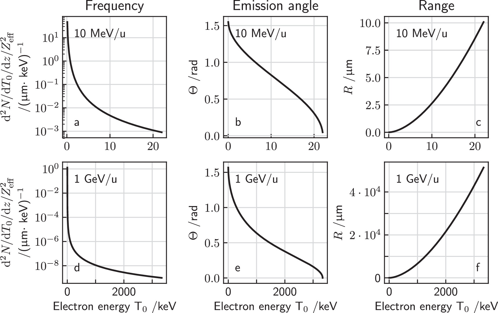
Figure 1. Energy spectrum, emission angle and range of secondary electrons as a function of their kinetic energy liberated by a 10 MeV u−1 (a)–(c) and a 1 GeV u−1 (d)–(f) ion. Note that through normalization of the frequency by  (a), (d) the production frequency becomes independent of the ion species.
Download figure:
Standard image High-resolution imageFrom equations (4) and (6) it is evident that each kinetic energy T is associated with a unique emission angle θ and a unique electron range R. Assuming a straight line-like propagation of the electrons in space, electrons stop at the surface of an almost ellipsoid shaped object directed in forward direction as visualized in figures 2(a) and (b) in a center plane cut through the track, where the lateral distance to the ion track is denoted by x.
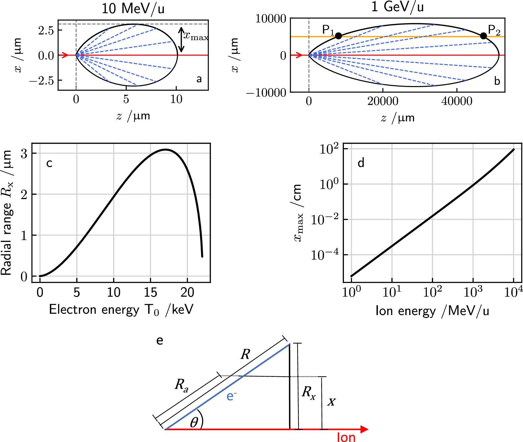
Figure 2. (a + b) section through the ellipse like boundary of the track structure developing from a point like secondary electron emission at (0, 0) for two ion energies. The electrons carry the energy outwards, forming the track structure. At a compromising energy the range and emission angle are large enough to reach the largest radial range  . For any given radial distance x only a limited angle and correspondingly kinetic energy interval refers to electrons passing that distance. (c) Radial electron range Rx
as a function of electron energy T0 for electrons liberated by a 10 MeV u−1 ion. (d) Maximum radial range xmax as a function of ion energy. (e) Sketch of the ion-electron collision kinematics: electrons get emitted at angle θ reaching a maximum radial range Rx
at the end of their range R.
. For any given radial distance x only a limited angle and correspondingly kinetic energy interval refers to electrons passing that distance. (c) Radial electron range Rx
as a function of electron energy T0 for electrons liberated by a 10 MeV u−1 ion. (d) Maximum radial range xmax as a function of ion energy. (e) Sketch of the ion-electron collision kinematics: electrons get emitted at angle θ reaching a maximum radial range Rx
at the end of their range R.
Download figure:
Standard image High-resolution imageThe maximum radial track extension  is reached at intermediate energies, compromising a fairly long range and a not too small emission angle. To determine it, one considers the distance perpendicular to the track

at which electrons of initial energy T0 come to rest, differentiates it with respect to T0 to find the energy resulting in the maximum distance and substitutes it in the expression for the distance. Although an analytic solution exists, it is lengthy and not educational. In approximation for nonrelativistic energies one derives

where E labels the specific kinetic ion energy (i.e. kinetic energy per nucleon). Figure 2(d) shows the dependence of the track radius on the ion energy. Strikingly, the range of track radii in the MeV/u region up to 1 GeV u−1 extends from μm to cm.
To determine the amount of energy that the δ-electrons carry away from the track center, we first consider the reduction of the secondary electron energy along their path. From figure 2(e) we find the relation of ranges

where at the left hand side the scaling between energy and range equation (6) has been used, and the remaining energy of an electron at distance x which originally had kinetic energy T0 is denoted as T(x, T0). Rearranging terms one obtains

In figure 3(a) examples are shown for the dependence of the kinetic energy at x depending on the initial kinetic energy. Notably, there are two limit cases, marked as points P1 and P2 in figure 2(b), restricting the range of emission angles resulting in a radial procession of the δ-electrons exceeding x. They correspond to two initial energies T0,1 and T0,2, and only initial energies between them refer to a large enough range and simultaneously a sufficient large angle emission that radial ranges larger than x are reached. They can be determined numerically as roots of the equation  . All kinetic energies electrons can have at distance x correspond to the range (T0,1; T0,2) of initial energies, as visible in figure 2(d).
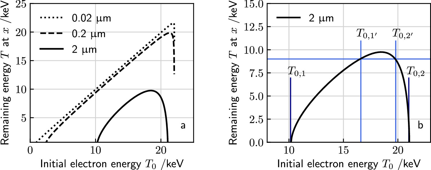
Figure 3. Remaining electron energy at different distances x to the track center in dependence on the initial energy (a). Quantities of interest in the relation between kinetic electron energies at distance x to the track center and initial energies. Only a limited interval of initial energies (T0,1; T0,2) corresponds to electrons passing the distance x. Considering an energy T > 0 remaining electron energy at that distance corresponds to an even more restricted initial energy interval  (b). In this example the incident ion's kinetic energy is 10 MeV u−1. Note that the quantities are independent of the ion species.
Download figure:
Standard image High-resolution imageTo obtain the radial dose profile, first of all the energy stored outside x per path length dz of the ion is expressed as

where the tilde indicates spectral weighting. The differential energy loss at radius x is then given as the derivative

which can be evaluated numerically, and the radial dose profile as

where ρ = 1 g cm−3 is the density of liquid water. The resulting profile is over many decades very well represented by a 1/x2 dependence as a reasonable fit by

Noteworthy, the quadratic decay of the dose from the inner parts of the track structure outwards does not follow from a simple geometric argument. Rather it is a subtle consequence of the spectral composition of secondary electrons and their energy loss properties. Hence equation (14) does not follow from an analytical derivation.
2.2. Track structure simulations with Geant4-DNA
The radial energy spectra calculated by the extended Kiefer–Straaten model are compared to corresponding spectra calculated with the Monte Carlo particle transport toolkit Geant4 (Agostinelli et al 2003, Allison et al 2006, 2016). The code extension Geant4-DNA is applied as it allows the step-by-step simulation of physical interactions (Incerti et al 2010a, 2010b, Bernal et al 2015, Incerti et al 2018) in contrast to the faster condensed history approach used in common Geant4 simulations. Furthermore, the common Geant4 models as well as FLUKA (Ferrari et al 2005, Böhlen et al 2014) have an electron production cut below which electrons are not produced. Instead the corresponding energy is deposited locally. Thus, these Monte Carlo codes are not suitable to validate the model results presented in this paper. However, also Geant4-DNA is limited in this sense since its electron interaction models are only available for electrons up to a kinetic energy of 1 MeV (Incerti et al 2018). Thus, simulation scenarios are limited to lower energetic ions whose secondary electrons carry a maximum kinetic energy below 1 MeV. Furthermore, model inconsistencies were found for ion ionisation models at ion energies >100 MeV u−1. Below this energy threshold (<100 MeV u−1) the systematics we observed are the same as visible at 10 MeV u−1.
The Geant4-DNA physics list option 2 is used, which provides a pre-selected set of cross section models. For light ions up to helium elastic interactions, excitations and ionisations are considered. For heavier ions only ionization processes are included. For the energy range of 500 keV to 100 MeV proton ionization processes are based on the Born and Bethe theories and the dielectric formalism for liquid water including relativistic effects and the Fermi-density correction. Below 500 keV a semi-empirical approach is applied to account for the deviation from the Born theory. This semi-empirical approach is also used for heavier particles (Dingfelder et al 2000, Incerti et al 2010a). In the case of electrons elastic, excitation, ionisation, solvation, vibrational excitation and attachment processes are simulated. Below the tracking cut of 7.4 eV the tracking of electrons is stopped and their remaining kinetic energy is deposited locally. For the simulation of radial energy spectra of secondary electrons, 5 × 10⁷ primary ions are tracked along the passage of 1 μm within water cube of 200 μm side length. All ejected secondary electrons are tracked down to their tracking cut (electrons of later generations are generated but not tracked). The electron spectra are then scored in cylindrical shells around the primary particle's track. In this manuscript the simulation results are shown for a 10 MeV proton and the scoring shells are set at 20 nm, 200 nm and 2 μm. To obtain the electron energy spectra, the kinetic energy of each electron is scored if it passes one of the defined shells during a simulation step as shown schematically in figure 4. This scoring is performed independent of the direction of the passage through a shell.
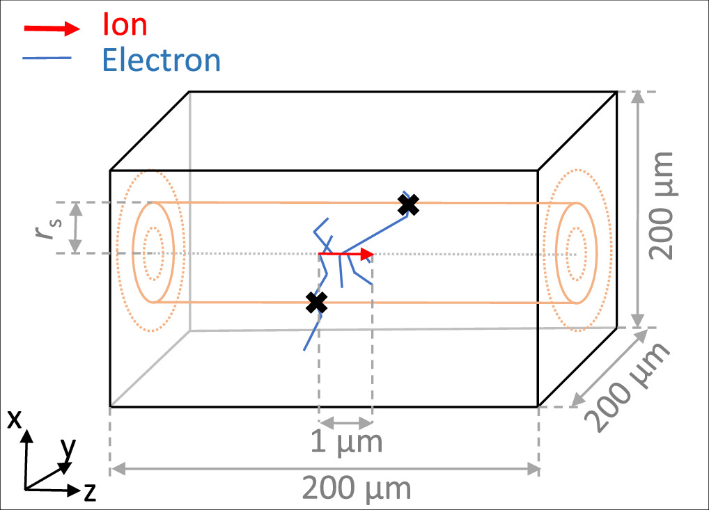
Figure 4. Sketch of the Monte Carlo geometry and scoring method for radial secondary electron spectra. The primary ion is created in the center of a water qube and its track is simulated along 1 μm (red arrow). All secondary electrons are tracked until they stop (blue lines). The energy of a secondary electron is scored in a histogram if it passes through cylindrical shells in defined distances rs to the ion track center (black crosses).
Download figure:
Standard image High-resolution image3. Results
3.1. Spectrum of secondary electrons
The spectrum of secondary electron kinetic energies at distance x to the track center is obtained by inspecting their dependency on initial electron energy as considered in figure 3. Remarkably, the remaining energy as function of the initial energy shows a peak. Hence, below the maximum remaining energy every specific value of kinetic energy corresponds to two initial kinetic energies, a small one with a large emission angle and a large energy with a small emission angle. Thus, the relative frequency of a remaining energy value has two contributions. If within a small considered interval of initial energy the remaining energy at distance x varies slowly with initial energy, the contribution of that energy to the spectrum will be large, and vice versa. Hence, the terms that need to be summed up for both contributing initial energies consist of the production cross sections for these energies multiplied with the modulus of the inverse derivative terms  :
:

This equation describes the translation from the initial electron kinetic energy spectrum to the one at distance x as visualised in figure 3(b). Here the evaluation energies  and
and  are the original kinetic energies leading to kinetic energy T at distance x. Technically, for a given distance x these initial energies have to be determined at first for the energy of interest. Then the initial spectrum weight at both energies has to be evaluated, and the derivative terms are obtained as the inverse of the derivative of equation (10), which then has also to be evaluated at the two initial energies. Finally all quantities can be expressed in terms of the remaining energy T. Note that equation (15) is evaluated numerically due to the complexity of the underlying functions.
The spectral composition at various distances x to the track center are displayed in figures 5(a) and (b) for 10 MeV u−1 and 1 GeV u−1 ions, respectively. To assess the general properties of track structure for these two example cases, some characteristic measures of the amorphous track structure description are summarized in table 1. As expected, the number of δ-electrons decreases rapidly with distance. The spectrum is peaked and shows a transition of the most prominent energies with distance: While close to the track center low-energetic electrons dominate the picture, in larger distances rather high energetic electrons occur. The distributions end with a strong peak at high energies. This is due to the maxima of the plots in figure 3(a), resulting in a mathematical singularity.
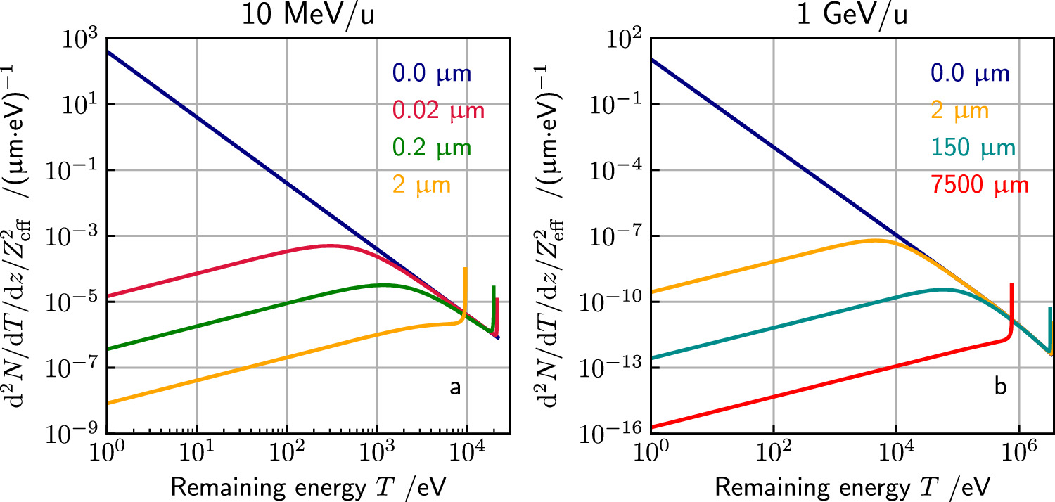
Figure 5. Spectral composition of δ-electrons at distance x to the track center for 10 MeV u−1 and 1 GeV u−1 ions. Note that through normalization of the frequency by  the production frequency becomes independent of the ion species.
Download figure:
Standard image High-resolution imageTable 1. Measures characterising track structure for 10 MeV u−1 carbon ions and 1000 MeV u−1 iron ions. Note that the given values only depend on the ion energy, but not on the specific ion type charge, i.e. 1000 MeV u−1 carbon ions would result in the same values as iron at that specific energy.
| 10 MeV u−1 | 1 GeV u−1 | |
|---|---|---|
| Maximum electron energy Tm (keV) | 22.06 | 3372 |
| Maximum range R(Tm ) (μm) | 10.12 | 52 314 |
Maximum lateral range  (μm) (μm) | 3.09 | 8623 |
| Energy of maximum lateral range (keV) | 17.03 | 2459 |
| Range at maximum lateral range (μm) | 6.52 | 30 586 |
| Emission angle with maximum lateral range | 28.3° | 16.4 ° |
Figure 6 presents the results of the Monte Carlo simulations for radial electron spectra. They largely reflect the course of the presented model except for very low (<200 eV) and high electron energies combined with large radial distances. For low energies, Monte Carlo results tend to be higher, indicating that the assumption of a continuous slowing down of electrons by means of equation (6) is not justified. There, few ionizations result in a strong scatter and terminate the directionality of electron propagation as predicted from the first generation ionization. Instead, for a sufficient number of interactions at higher energies the continuous slowing down approach reflects the average projected range reasonably well, as the parametrization equation (6) is derived from experimental data of such energies. However, still the directionality is lost and only given in the statistical limit over many electron tracks. At the high energy end, the MC results predict electrons with even higher kinetic energy than allowed by the model, which becomes in particular visible at large lateral distances (see the yellow curve for 2 μm distance). This again can be attributed to the assumption of straight line propagation in the amorphous track model. If this is violated by individual scattering events, and in general an energy dispersion is expected, leading to a smear-out of the singularity predicted by the analytical model.
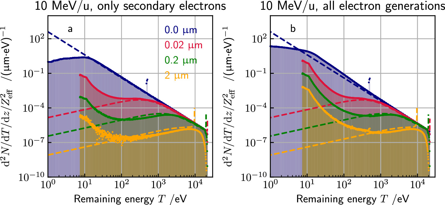
Figure 6. Spectral composition of δ-electrons at various radial distances x to the track center calculated by the analytical model (dashed lines) as well as computed with Geant4-DNA simulations (histograms). The peak in the blue curve at about 500 eV in the MC simulations refers to Auger electrons. The Monte Carlo simulations are performed only scoring secondary electrons (a) and scoring all electron generations (b). The analytical calculations (dashed lines) are the same in both panels and refer to only secondary electrons.
Download figure:
Standard image High-resolution image3.2. Radiation quality across the track structure
The detected turnover from most prominent low to large remaining electron energies clearly demonstrates that also radiation quality (i.e. the spectral composition) and not only energy deposition (i.e. local dose or specific energy) varies across the track. To characterize this feature we here consider the electron LET. Starting from equation (6) one can equate the LET by

resulting in a decrease of LET with T−0.7. Figure 7(a) shows the LET as a function of the kinetic electron energy.
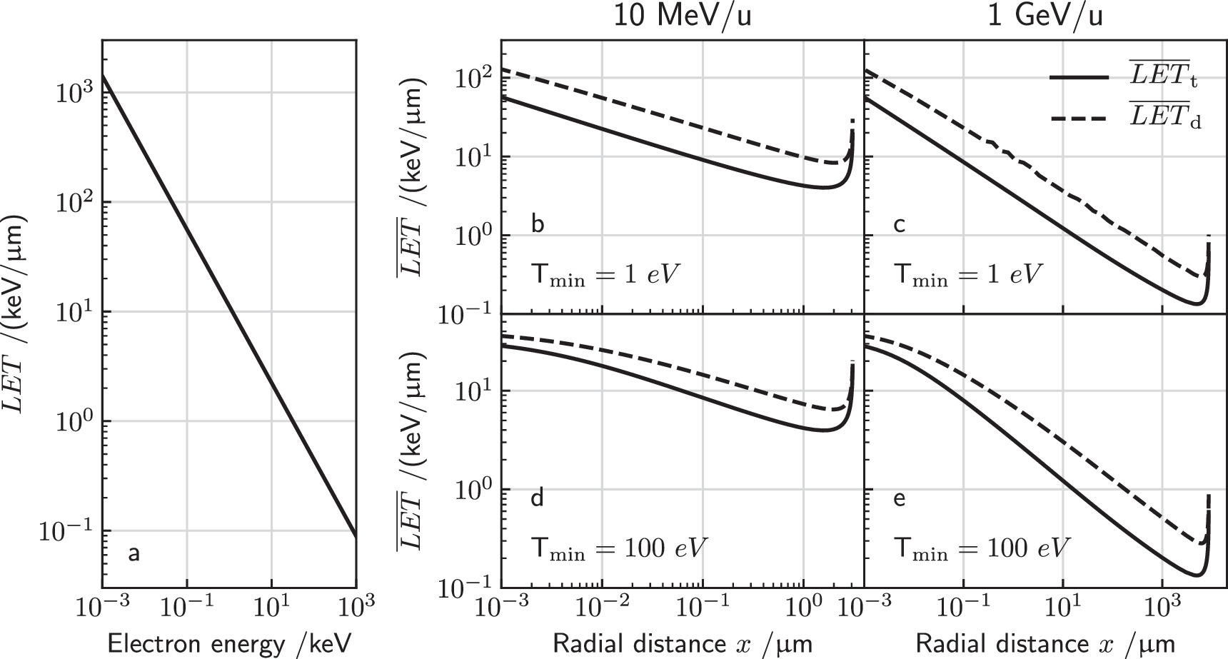
Figure 7. (a) Electron LET as a function of kinetic energy. (b)–(e) Track and dose mean LET at radial distance x are shown for 10 MeV u−1 and 1 GeV u−1 ions in the left and right panels, respectively. Two different values for Tmin are selected as given in each panel.
Download figure:
Standard image High-resolution imageAdopting an approximate W-value of W = 34 eV (the energy on average spent per ionization, including other losses like excitation) this can be converted in the average number of ionisations per length segment, and the average spacing between two adjacent ionisations on the electron track is given by

At low energies in the order of 1 keV the average distance meets the nanometer scale and eventually the electrons form track ends, where ionisations occour even more dense and hence the formation of double strand breaks is fostered. In contrast to that, the formation of such lesions by means of multiple electron processes becomes important only at very high local doses (Friedrich et al 2015).
While these considerations hold for monoenergetic electrons, in a real irradiation scenario the spectrum of electron energies has to be taken into account. As usual for ion radiation we define the track and dose averaged LET as

and

Here  is the maximum remaining energy occurring in the spectrum, which can be determined numerically by finding the maximum of equation (10). The lower integration limit Tmin has to be chosen reasonably because with the continuous slowing down expression equation (16) the LET will diverge towards zero energy, leading to a divergence of the integral. Both LET measures are visualized in figure 7. A plausible value for the integration limit is in the order of 10 eV or a few 10 eV according to ionization threshold in water or other considered target materials.
Notably, both LET measures fall off with distance x to the track center with a final peak at the track ridge. Within the model we find a scaling alike LET ∝ x−0.4, which can be reasoned analytically as outlined in appendix C. At the maximum track width, however, the LET runs into a singularity, as there essentially all electrons have dispensed their kinetic energy, and only comparably low-energetic electrons with high electron LET are left.
The LET pattern within a track structure depends only on the ion energy but not on the ion type, because the ion charge only appears as a prefactor in the spectrum equation (1). As the spectrum is used as weighting factor occurring both in the numerator and denominator in equations (18) and (19), the charge dependence cancels out.
The model results also show that the low energy integration limit the LET towards low distances x, where low-energetic electrons are particular prominent. At larger distances this impact vanishes gradually, where the impact on LETd remains more persistent than for LETt .
The LET is often considered as a predictor for the biological effectiveness, as it specifies the local energy loss, which is the origin for local DNA damage formation. Large LET values imply an increased formation of complex damage. The results indicate that DNA damage production is most effective in the center region of ion tracks.
3.3. Electron build-up effect
When ions enter from vacuum (e.g. from an accelerator beamline) into matter, an electron dose build-up effect is observed. Due to the dominance of forward scattered electrons, there is no equilibrium between energy carried away and inferred by secondary electrons within the first mm of the material. Hence, a build-up region of dose is established and its longitudinal length is essentially given by the maximum range of secondary electrons.
Within the here presented model the energy and angle distribution of secondary electron emission are accessible and, thus, the shape of the build-up can be determined analytically, as outlined in the following. In accordance to equation (10) the remaining energy when an electron has passed the longitudinal distance z is given by

with the longitudinal electron range  . With that the energy deposition at depth z can be calculated as

with

where the cosine term in the denominator of the integral kernel k(z) converts the LET as energy loss per path length into energy loss per longitudinal procession. The integration space encompasses all possible depths of electron production which reach position z. Therefore, a distinction has to be made between low-energetic electrons which need to be produced close enough to z in order to have a range beyond z (first integral), and high energetic electrons that have a large enough range to reach z wherever they are produced (second integral). These cases are separated at energy T1 which is the energy, where the longitudinal range is just z, i.e.  . Note that the first integral has a lower bound at
  which is essentially given by the ionization thresholds.
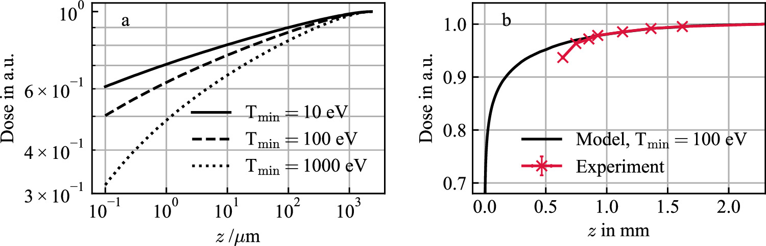
Figure 8(a) shows calculations of the electron build-up for three values of  . The analysis confirms that the spatial expansion of the build-up effect is defined by the range of the electrons. The extent of the effect depends on the minimum energy
  . If a higher energy cutoff is chosen, not allowing for the production of low-energetic electrons, the fraction of electrons with larger range is higher and hence the 'dose hole' at the interface into material seems broader. In particular that means, that the build-up effect is strongly depending on the target material, i.e. on its charge number Z, which scales the mean ionization threshold.
Figure 8. Dose build-up effect due to pronounced forward scattering of secondary electrons for three cutoff energies  for 220 MeV u−1 ion irradiation (a). Comparison of the simulated build-up effect to measurement data taken from Pfuhl et al (2018) (b). In the experiment the distance between the beam exit window and the first ionisation chamber was 64 cm, which corresponds to a water equivalent thickness of d ≈ 0.64 mm. Thus, for the experimental data points, all z values were shifted by d to be able to compare them to the analytical model. The measurements were performed with polyethylene and were converted to water-equivalent thicknesses in (b). All curves are normalized to 1 at the maximum electron range.
Download figure:
Standard image High-resolution image
In figure 8(b) the model predictions are compared to experimental measurement data taken from Pfuhl et al (2018). Both build-up curves are normalized to a material thickness corresponding to the maximum electron range for 220 MeV incident protons (≈2.3 mm). The general trend of the model matches the experimental findings. However, it needs to be considered that the ionization chambers used for the measurements of the build-up curves have a limited size in contrast to the model calculations. The absolute measured dose directly depends on the size of the active area of the ionization chamber (Pfuhl et al 2018). Furthermore, any air gap, foils at the beam exit window or within the ionization chamber influence the shape of the measured dose build-up curve.
4. Discussion
4.1. Model limitations
In this work we applied the track structure theory of Kiefer and Straaten to analyze the secondary electron kinetic energy spectra in arbitrary distance to an ion track center. The notion of an amorphous track structure brings along a number of limitations as a consequence of the underlying assumptions:
- (i) A continuous transfer of energy from the ion to δ-electrons is assumed, ignoring the stochasticity of that process.
- (ii) Likewise, in reality the electrons lose their energy in quanta via ionization and excitation processes instead of continuously, as assumed. However, this is not a unique assumption in amorphous track structure models but also applies to the definition of LET.
- (iii) The assumption of linear electron propagation is crucial. As in realistic electron tracks the projected range which determines the track structure width differs from their trajectory range by means of multiple momentum changes, energy-angle correlations will be softened. This becomes in particular important at low kinetic energies and results in the deviation between the Monte Carlo and the continuous slowing down approach in figure 6. However, we checked that the fraction of initially ionized electrons with such low kinetic energies (<100 eV) is a few percent only. For higher energies the power law of equation (6) reflects range measurements sufficiently well (see figure A4 of ICRU 1970).
- (iv) The model does not make any statements about the track center. For instance equation (3) can not hold there because then the energy integral over the entire track would not converge, violating conservation of energy. Rather a flattening of the dose profile at the track center is expected (Krämer 1995).
- (v) The model neglects the formation of second generation electrons, but only considers the corresponding energy loss. However, these electrons have typically small energies but nevertheless might give rise to one or few further ionisations, potentially distorting the graphs for all spectral weighted quantities.
- (vi) The empiric expression for the electron range due to collision losses is only valid for electrons up to about 1 MeV kinetic energy. Above this gradually loses validity, and in addition bremsstrahlung losses become important, so that the electron LET is increasing again. However, as only a small fraction within the δ-electron spectrum assumes such high energies this is usually not a matter of concern (see figure 1(d)). Also, the energy-range scaling is not valid for low-energetic electrons which are about to stop.
- (vii) In the regime of low momentum transfer, the binding energy of electrons is neglected.
- (viii) In general, numerous corrections to the Bethe equation are also ignored here. However, they usually do not affect the energy region of interest for the δ-electrons.
Some of these limitations can be at least partially overcome by detailed Monte Carlo transport calculations (Chatzipapas et al 2020). They agree—just as various amorphous track structure formulations do—in the quadratic decay of dose with increasing radius within the track, but differ in the shape and magnitude of the radial dose profile close to the track center (Cucinotta et al 1999, Elsässer et al 2008, Wang and Vassiliev 2017). However, at that point it is important to note that the Monte Carlo codes have their limitations as well. They depend on (i) the level of detail included, (ii) the physical interaction processes taken into account, (iii) the associated cross section data and (iv) cut off energies. Cross sections typically have considerable uncertainty in particular at low energies, which explains partially the variability among the codes in the track center. The lack of reliable cross section data is a direct consequence of the limited experimental accessibility in that regime.
As a consequence, all state of the art approaches have some uncertainties in accounting for the low energetic portion of secondary electron spectra. However, these uncertainties do not prevent an application within effect models, as on the other hand also experimental data have intrinsic uncertainties. Taking spectral properties within the track structure into account may be despite associated uncertainties helpful to assess the expectation values of radiobiological effects correctly.
4.2. Amorphous track structure in radiobiological effect modelling
Amorphous track structure models are easy to use and allow simple mechanistic insight without the need of simulating individual electron tracks in time-consuming transport calculations. The limitations listed in the previous section indicate that such models reflect the general properties of energy deposition in the sense of dose while ignoring the stochastic nature of energy deposition. The simplicity of amorphous track structure models allows their uncomplicated exploitation to explain and predict the RBE of ion radiation. These models have in common, that the dose response to low-LET radiation with a homogeneous exposure across the cell nucleus is extrapolated towards the response to high-LET radiation. While all models rely on the quadratic decrease of dose with distance to the track center, the applied amorphous track structure formulations differ in the dose present in the ion track center. Unfortunately, due to the small relevant spatial scales, no measurements are available in that region and only Monte Carlo studies give indications about its physical properties (Krämer 1995). In this work no assumptions about the track structure in the interior of the track is made. Therefore, dose integrals over the track structure do not converge, which is, however, not the focus of the present work.
The concept of amorphous track structure was introduced for the purpose of RBE modelling within the Katz model (Butts and Katz 1967). While that model was even simpler than the Kiefer–Straaten approach by only considering electron propagation perpendicular to the ion path, it already succeeded to predict the quadratic dose decay with distance to the track center. However, the associated Katz model for predicting the RBE (Butts and Katz 1967) only considers local dose but ignores its the spectral composition. Likewise in the microdosimetric kinetic model (MKM) (Hawkins 1996, Inaniwa et al 2010) which is involved in treatment planning in several carbon ion cancer therapy facilities only local energy deposition within microdosimetric domains of the order of a micron are considered, but not the underlying spectral composition of electrons. In the LEM, the Kiefer–Straaten model is used to determine the local dose as the expectation value of energy concentration anywhere within cell nuclei. The inner part of the track structure is assumed to be constant such that the local dose transitions continuously into the quadratic decay portion of the track structure. Furthermore, the dose integral over the entire track structure is defined to reflect the total deposited energy as given by the LET. Hence the prefactor in equation (14) becomes energy-dependent. While over the years, the LEM was gradually improved to include aspects like the action mediated by radiolysed radicals or double-strand-break (DSB) proximity, the spectral electron composition had not been considered, yet.
Per unit dose, DSB induction may be enhanced for ions as compared to low-LET radiation by two distinct processes: (i) at high doses any two secondary electrons may induce a DSB jointly by inducing SSB at opposite strands of the DNA in proximity. This effect was included in the LEM since version II. And (ii) individual low-energetic electrons have an enhanced efficacy in inducing DSB. Concerning the latter, the presented model provides the opportunity to include the spectral information of secondary electrons in RBE models. In combination with a DSB induction model, which provides the secondary electron RBE as a function of their energy (Pfuhl et al 2022b) more precise RBE predictions can be performed. For this purpose an average electron RBE is determined as a function of the radial distance to the track center by weighting the electron spectra with the electron RBE. Then, the dose profile obtained from an amorphous track structure model can be weighted with the average electron RBE. This concerns all RBE models that are based on a track structure model such as the Katz model, the MKM or the LEM. This new feature was recently implemented into the LEM V, and a corresponding publication is in preparation. In the framework of microdosimetry the method presented here could lead to corresponding adjustments in weighting function approaches.
The inclusion of spectral electron information led to improved RBE predictions in particular for high-energetic carbon ions. The corresponding publication is in preparation. Additionally, in the same context this approach might give an insight in understanding the origin of the increased RBE for protons in the entrance channel of radiation fields. In fact, an RBE typically exceeding 1 is observed for high-energetic protons (Paganetti 2014). This is remarkable, as the dose profile is often referred to be 'photon-like' since the local doses are low and their distribution is broad. However, the secondary electron spectra of photons and protons differ with a larger fraction of low-energetic electrons in the case of protons. The above described approach allows to include the increased effectiveness of the more prominent low-energetic electrons in the RBE determination and, therefore, might be a valuable key to understanding the increased RBE of high-energetic protons.
Finally, the underlying strategy to employ a spectral weighting of effectiveness once the spectral composition within an ion track structure is known can be generalized to arbitrary radiation fields, also other than ion tracks. The small secondary electron energies of ultrasoft x-rays have been attributed to their observed enhanced effectiveness (Goodhead and Nikjoo 1989). Likewise, the low energies compared to orthovoltage x-rays in the spectrum of mammography x-rays with maximum energy of about 30 keV are considered to be pivotal for their enhanced effectiveness (Nikjoo and Lindborg 2010).
4.3. Spectral properties of track structure
The analysis presented in this work shows that the energy spectra within the ion track structure are typically broad. Additionally, the most prominent part of the spectrum transitions from low to rather high electron kinetic energies with distance to the ion track center. This is counter-intuitive at the first glance, as it is in seeming contrast to the energy loss, but is understandable by considering the large production rates along with small ranges of low-energetic electrons. The shape of the spectra are largely supported by MC simulations, albeit in these individual electron propagation is considered, including elastic scattering and further ionization processes. This supports the validity of amorphous track structure models also in an energy-resolved perspective.
Because of the higher biological efficacy of low-energetic electrons a variation of effectivity across the track structure is expected, as indicated by the LET variation. In the present work these results were found solely based on amorphous track structure. They also confirm findings published in Nikjoo and Goodhead (1991) highlighting the importance of low-energetic electrons for both dose and effectiveness. A study by Cucinotta et al (1999) used energy dependent electron RBE values along with precalculated electron energy distributions to determine the RBE within a track as function of the track center distance came to a similar conclusion. There, also after an initial drop of electron effectiveness with increasing radius, a recovery towards the maximum track radius was predicted, which is expected from track ends formed by outermost electrons. From the results presented here we considered the integral of the LET-weighted dose across the track structure including or excluding the rise towards the singularity and found a difference in the order of a few percent. As this quantity serves as a first order predictor of biological effects, this indicates that the recovery may contribute to the overall effect to a non-negligible extent, depending on the regarded endpoint and desired uncertainty.
The biological effects of ion tracks depend on one hand on the energy concentration within the track structure, i.e. the local doses, but as well as the lesion production per dose. The latter aspect is impacted by the spectral radiation composition, but there are practically no data where this impact can be investigated isolated from other factors. However, in DSB yield measurements by gel electrophoretic elution a trend towards larger yields was detected after irradiation with high energetic ions as compared to photon radiation (Taucher-Scholz et al 1996). This finding is not expected for such high ion energies since for such large ion tracks a dose bath similar to photon radiation is found. In such cases many ion tracks overlap to reach even small macroscopic doses and thus, the prominence of large local doses in the ion track center decreases. In fact, this could be a fingerprint of a shift in the secondary electron spectrum in comparison to that of photon irradiation, including a higher proportion of low-energetic electrons in the case of ion radiation.
Concerning physical doses, the findings from investigating the build-up effect suggest a material dependence, as the charge number Z of target atoms essentially scale their ionization potential. Here one has to keep in mind that measured dose profiles exhibit a dose build-up effect that reflects to some extent the properties of the surroundings, e.g. foils in the measurement chamber and ambient air gaps or water. However, corresponding electronic build up effects find their saturation within the scale of a mm in water, and hence a small bolus in front of the accelerator exit window is a pragmatical solution to warrant electron equilibrium in the ionization chamber and the biological target material.
5. Conclusion
This document presents an approach for the derivation of secondary electron spectra as a function of the radial distance to ion track centers. It is based on an amorphous track structure model by Kiefer and Straaten and confirms that the composition of δ-electrons varies within the ion track structure, showing the prominence of high-LET components in the interior parts. Furthermore, after an initial decrease of LET with the radial distance, a final increase is found at the rims of ion tracks. Hence, the radiation quality varies considerably across the ion track, which indicates that the inclusion of this effect in RBE predictions of ions leads to more precise results. In this context the presented model for secondary electrons is applied in the future implementation of the LEM. Combined with an electron RBE model the average electron RBE can be determined as a function of the radial distance to the ion track. In combination with an amorphous track structure model to describe the local dose profile in an ion track this leads to improved ion RBE predictions, especially for high energetic ions.
Acknowledgments
This work was supported by HGS-HIRe for FAIR (Helmholtz Graduate School for Hadron and Ion Research).
Data availability statement
All data that support the findings of this study are included within the article (and any supplementary information files).
Appendix A.: Derivation of equation (3)
An ion passing an electron (assumed to be at rest initially) at impact parameter b causes a transient force on the electron, resulting in a momentum transfer. The momentum the electron gains is estimated from the time integration of the Coulomb force component perpendicular to the ion motion and reads

where Z refers to the ion charge number, e is the elementary charge and  0 the vacuum permittivity.
The relativistic energy–momentum relation allows to express the kinetic energy of the electrons as

while a classical calculation would rely on T = p2/2me (not followed in this work). Together with the previous equation a relation between b and T is given.
The number of electrons at impact parameter b in a thin cylindrical shell of thickness db and length dz can be written in terms of the electron number density n as

Using the above relation between b and T we obtain

where the last step includes some elementary algebra. The ion charge number is finally replaced by the recombination corrected effective charge Z*.
The electron number density can be written as

where NA is Avogadro's constant, mM is the molar mass of the target material (here water), ΣZt is the summed charge numbers in target molecules, and ρ is the target mass density.
In comparison with equation (3) the prefactor equates to

where α is the Sommerfeld fine structure constant and ℏ is Plancks constant. Inserting NA = 6.023 × 10²³mol−1, α = 1/137, ℏ c = 197 MeV fm, me c2 = 511 keV, ΣZt = 10, mM = 18 g mol−1 and ρ = 1 g/cm3 results in C ≈ 8.5 eV/μ m.
Appendix B.: Derivation of equations (4) and (5)
Consider an ion with kinetic energy T and momentum vector p interacting elastically with an electron at rest. Let after the collision process the ion have energy  and momentum vector
  , and the electron
  and
and  , respectively, where the dash labels quantities after the collision and the index e labels the quantities referring to the electron. Then conservation of energy and momentum imply


Solving the momentum equation for  and squaring leads to

where θ is the deflection angle of the electron caused by the interaction process. Expressing the energy and momentum equations in relativistic parameters results in


Using the identity γ2 − 1 = β2 γ2 this can be simplified to


with the ratio of electron to ion mass f = me
/M. Inserting the first into the second equation to eliminate  allows to establish a relationship between electron kinetic energy (depending on
  and the scattering angle θ. After some elementary algebra we obtain

In the limit case of knock-on collisions, i.e. for θ = 0, the cosine term becomes 1. Then the electron kinetic energy is the maximum possible energy transfer and can be equated, as usual, by solving for  and calculating the kinetic energy as
  . This results in

which is just equation (5).
In general, equation (31) can be transformed into

By using  to replace
  and by using equation (B9) to replace the f-dependent terms one finally arrives at equation (4).
Appendix C.: Derivation of the scaling property of LET
It has been shown within the model that both LET measures, LETt and LETd decrease with x−0.4. This behaviour shall be reasoned in the following.
In the spectra of remaining energy figure 3 the cross sections essentially drop as T−2 for the gross part of the spectrum. The low energies for which this is not true are rather rare and only resolved due to the logarithmic scale in the figure, and the very high energies which eventually form the singularity also cover a small fraction of all integrals, as can be checked by comparing integrals over the cross sections including or excluding the rising part towards the singularity. Hence we can assume d2 N/dTdz ∝ T−2. The LET can be derived from equation (6) as LET = T1−a /(aK), and hence the expressions for LETt and LETd become

and

The integration limits cover the relevant spectrum of electrons at distance x, where for not too large distances the upper limit T2 is of the order of Tmax, so that T2 ≫ T1 holds and the terms with T2 can be neglected. The lower integral boundary marks the remaining energy from which on the frequency distribution is in accordance with the ∝T−2 scaling. Considering that in equation (15) the first term usually dominates due to higher cross sections and larger derivative terms, this implies that the derivative term dT0/dT is of the order of 1. In figure 3 it is visible that the remaining energy curve starts from 0 and approaches quickly that regime, so the minimum remaining energy we search for as integration limit can be approximated by the minimum original energy of electrons reaching distance x. Considering equations (6) and (7) the sine term can be set to 1 for the small energies (i.e. for almost perpendicular secondary electron emission) and the minimum energy can be found by  , solving for
  . Inserting this into the integrals results in

and

The decay exponent evaluates to (1 − 1/a) ≈ 0.41 which reflects the model findings.