

Abstract
Objective: pulsed fields or waveforms with multi-frequency content have to be assessed with suitable methods. This paper deals with the uncertainty quantification associated to these methods. Approach: among all possible approaches, the weighted peak method (WPM) is widely employed in standards and guidelines, therefore, in this paper, we consider its implementation both in time domain and frequency domain. For the uncertainty quantification the polynomial chaos expansion theory is used. By means of a sensitivity analysis, for several standard waveforms, the parameters with more influence on the exposure index are identified and their sensitivity indices are quantified. The output of the sensitivity analysis is used to set up a parametric analysis with the aim of evaluating the uncertainty propagation of the analyzed methods and, finally, also several measured waveforms generated by a welding gun are tested. Main results: it is shown that the time domain implementation of the weighted peak method provides results in agreement with the basilar mechanisms of electromagnetic induction and electrostimulation. On the opposite, the WPM in frequency domain is found to be too sensitive to parameters that should not influence the exposure index because its weight function includes sharp variations of the phase centered on real zeros and poles. To overcome this issue, a new definition for the phase of the weight function in frequency domain is proposed. Significance: it is shown that the time domain implementation of the WPM is the more accurate and precise. The standard WPM in frequency domain has some issues that can be avoided with the proposed modification of the phase definition of the weight function. Finally, all the codes used in this paper are hosted on a GitHub and can be freely accessed at https://github.com/giaccone/wpm_uncertainty.
Export citation and abstract BibTeX RIS

Original content from this work may be used under the terms of the Creative Commons Attribution 4.0 licence. Any further distribution of this work must maintain attribution to the author(s) and the title of the work, journal citation and DOI.
1. Introduction
Human exposure to electromagnetic fields (EMFs) is regulated by different international standardization bodies such as the IEEE International Committee on Electromagnetic Safety (ICES) Technical Committee (TC) 95 and the International Commission on Non-Ionizing Radiation Protection (ICNIRP). They both provide safety guidelines and standards to avoid overexposure to EMFs (ICNIRP 2010, Bailey et al 2019). These guidelines propose exposure limits as a function of the frequency for the general public and workers. Although these limits are based on the up-to-date scientific literature, the development of new electric and electronic systems requires updates of these guidelines considering recent progresses (Hirata and Reilly 2016), future perspectives (Hirata et al 2021) and/or possible known gaps to be covered (ICNIRP 2020).
The interaction between EMFs and living tissues varies with the frequency. For instance, in the low frequency range (i.e. f < 100 kHz) the main effect is the interaction with the nervous system, whereas, in the high frequency range (i.e. f > 10 MHz) the main effect is the energy absorption causing heating of tissues (ICNIRP 2010). For frequencies that are in between the two ranges (i.e. 100 kHz < f < 10 MHz) the predominant effect must be verified case by case. However, it is worth noting that it is not always possible to reduce the problem to a single frequency exposure. In case of pulses or waveforms with multi-frequency content, the above mentioned limits must be coupled with a suitable approach that is able to take into account the complete spectrum of the field (Jokela 2000, ICNIRP 2003). Each standard and guideline addresses this problem differently proposing solutions that depends on the shape of the waveform (ICNIRP 2003, 2010, Bailey et al 2019). The literature includes several papers using these methods to analyze specific exposure scenarios (Lodato et al 2012, Andreuccetti et al 2013, Fiocchi et al 2015, Canova et al 2016, Paffi et al 2016, Giaccone et al 2020, Tang et al 2022) and other papers pointing out issues and performances of these methods (De Santis et al 2013, Schmid and Hirtl 2016, Keller 2017, Schmid et al 2019). Most of these methods move the problem from the time domain to the frequency domain by means of the Fourier decomposition of the waveform. In this way, each spectral line can be compared to a well defined limit that, as already mentioned, depends on the frequency. In a single frequency exposure scenario, the accuracy of the result depends only on the method used to measure or to compute the quantity to be assessed. In the case of pulsed or multi-frequency exposure, also the method of assessment increases the uncertainty of the final result because it involves other computations aimed to define an exposure index (usually a scalar value) that depends on the information coming from all the spectral content of the waveform and also on the implementation of the method. The literature cover comparisons between methods pointing out their strengths and/or weaknesses. For instance, De Santis et al (2013) consider most of the available methods proposed by the ICNIRP and the IEEE for the assessment of pulsed fields. Distinction between time-domain approaches and frequency-domain approaches is given and the stability of these methods is analyzed by considering the effect of noise, dc offset and truncation. The authors also propose a new method that should take the best from the time-domain approaches and the frequency-domain approaches. Unfortunately, this method was already proposed by Chadwick (1998) and it misses some important electrophysiological considerations as pointed out by Jokela (2000) that, for this reason, proposed improvements leading to a new method called weighted peak method (WPM). The WPM has been then included also in the ICNIRP guidelines (ICNIRP 2003, 2010). Schmid and Hirtl (2016) analyze the inconsistency of a time domain method that is included in the non-binding guide to good practice for implementing Directive 2013/35/EU (European Commission 2016) and originally proposed by Heinrich (2007). This method is compared with the results obtained with the WPM showing that it violates the underlying principle above which reference levels and basic restrictions are defined and, for these reasons, it should be avoided. Keller (2017) provides a thorough analysis of the WPM addressing many technical details for its implementation both in frequency domain and in time domain. The analysis shows that the WPM is the approach more closely related to the underlying concepts of electrostimulation and the results obtained are very reliable, especially when applied in the time domain. Schmid et al (2019) take into account 12 different time domain signals of magnetic field to test the methods proposed by the European Directive 2013/35/EU. They confirm the stability of the method proposed by the ICNIRP (i.e. the WPM).
In the literature, to the best of the author's knowledge, there is no study trying to evaluate the uncertainty propagation of any of the available methods. For this reason, in this paper the analysis of the uncertainty associated to the methods used to assess a pulsed or a multi-frequency field is considered. The polynomial chaos expansion (PCE) theory (Sudret 2008, Eldred 2009, Kaintura et al 2018) will be exploited first to perform a sensitivity analysis with the aim to identify the parameters with more influence on the final result. The PCE technique is very flexible and it has already been used in the context of human exposure to EMFs (Chiaramello et al 2017, Fiocchi et al 2018). Afterward, each parameter is analyzed within a reasonable range and, for each value of the parameter, the uncertainty propagation is evaluated by means of the PCE method obtaining mean value and standard deviation of the output quantity provided by the assessment method, that is the exposure index. Results will be presented as 95% confidence interval plots. It must be stressed that the method used for the uncertainty quantification is very general and it can be applied to all methods for the assessment of pulsed or multi-frequency fields, however, in this paper we take into account only the weighted peak method proposed by the ICNIRP because it is recognized to be the most suitable and less conservative among all methods (Schmid and Hirtl 2016, Keller 2017, Schmid et al 2019). The WPM can be applied both in time domain and frequency domain. Both approaches are considered and, furthermore, a modification in the implementation of the WPM in the frequency domain is proposed with the aim of improving its accuracy/precision.
Finally, for the sake of reproducibility, all the codes used in this paper are hosted on a GitHub repository that can be freely accessed at https://github.com/giaccone/wpm_uncertainty.
2. Materials and methods
2.1. Uncertainty quantification
Uncertainty quantification (UQ) is the process of determining the effect of input uncertainties on response metrics of interest (Eldred 2009, Kaintura et al 2018). In this paper the UQ is carried out using an analysis of variance (ANOVA) technique. An ANOVA method makes it possible to decompose the variance of the output as a sum of contributions of each input variable, or combinations of them (Sudret 2008). For instance, for a model function y of two parameters p1 and p2, the function can be written as

It is possible to show that the total variance of the output variable y can be defined as

where the terms on the right hand side are the partial variances depending on single parameters or a combination of them. In this paper, the variance terms are computed using the PCE approach (Sudret 2008). In particular, a free and open source PCE implementation developed by the author is used (Giaccone 2018). The tool has already been tested and validated in another context by comparing the results with the more standard (an time consuming) Monte Carlo method (Giaccone et al 2020).
In this section a short recall to the theory behind PCE is given. In PCE, the variation of the output on the inputs is projected on a set of multivariate orthogonal polynomials ψ. The uncertain parameters are here represented in matrix notation using the bold variable ![${\boldsymbol{p}}=\left[{p}_{1},{p}_{2},\cdots ,{p}_{n}\right]$](https://content.cld.iop.org/journals/0031-9155/68/9/095001/revision2/pmbacc924ieqn1.gif) . Both the output y and the orthogonal polynomials ψ are function of the uncertain parameters
p
and the the relation between them is given by
. Both the output y and the orthogonal polynomials ψ are function of the uncertain parameters
p
and the the relation between them is given by

where αj are coefficients and M is the order of the approximation truncated for computational reasons. The multivariate orthogonal polynomials ψj must be selected in relations to the distribution of the uncertain parameters according to the Wiener–Askey scheme (Eldred 2009, Kaintura et al 2018). For instance, the family of one-dimensional Hermite polynomials are suitable to represent an uncertain input with normal distribution. There are several approaches to determine the coefficients αj like linear regression and spectral projection (Sudret 2008, Eldred 2009, Kaintura et al 2018), in this paper the latter is used. By knowing the PCE coefficients αj in equation (3) it is straightforward to evaluate mean value (μ) and standard deviation (σ) (Sudret 2008, Kaintura et al 2018). They can be computed as


Finally, in order to evaluate the precision of the methods for assessing pulsed fields, the 95% confidence interval is used. For a given data set characterized by mean value μ and standard deviation σ, the 95% confidence interval is a range defined as ![$\left[\mu -1.96\ \sigma ,\mu +1.96\ \sigma \right]$](https://content.cld.iop.org/journals/0031-9155/68/9/095001/revision2/pmbacc924ieqn2.gif) . The range is centered on the mean value μ and the width is 3.92 σ. In the following, it is important to keep in mind that a confidence interval with narrow width corresponds to a high precision associated to the method analyzed.
. The range is centered on the mean value μ and the width is 3.92 σ. In the following, it is important to keep in mind that a confidence interval with narrow width corresponds to a high precision associated to the method analyzed.
2.2. Sensitivity analysis
The knowledge of the coefficients αj in equation (3) enables the computation of the variance (V) of the variable y related to the uncertain parameters p (Sudret 2008). Since equation (3) can be considered as a decomposition of the effect of each uncertain parameter in the output variable y, also partial variances can be computed (Sobol' 2001, Sudret 2008). The knowledge of partial variances allows to define Sobol' sensitivity indices as

Sobol' indices provide information about how much the variance of the output is dependent on a given input or a combination of them. For instance, for the output variable defined in equation (1), the Sobol' indices S1, S2 and S12 can be defined. Moreover, according to equation (6), the sum of all Sobol' indices related to a certain output variable is always 1. Bearing all this in mind, the higher the Sobol' index is, the higher is the influence of the related variable on the variance of the output.
2.3. Analysis of pulsed fields
In this paper the weighted peak method is considered for the assessment of pulsed fields (Jokela 2000, ICNIRP 2003, Keller 2017). Given the variable A(t) that can ben either an external field (electric or magnetic) or an internal/induced quantity (electric field). The WPM is described by the following equation

where fj is the jth frequency of the spectrum, Aj is the amplitude of the jth component of the spectrum of A(t), θj is the phase of the jth component of the spectrum of A(t), WFj is the amplitude of the weight function and it is defined as the inverse of the peak limit at the frequency fj , φj is the phase of the weight function at the frequency fj and it is defined with rules provided in the ICNIRP guidelines (ICNIRP 2003, 2010). EI is the exposure index that, for compliance, must be lower than 1.
The WPM can be applied both in time and frequency domain (Jokela 2000, ICNIRP 2003, 2010, Keller 2017). In the author opinion, the ICNIRP guidelines provide a misleading description of the relation between the two implementations. Since each limit is defined in the frequency domain, the ICNIRP guidelines provide, at first, a description of the implementation of the WPM in frequency domain. Then, the implementation in time domain is literally described as an approximation of the WPM in frequency domain (ICNIRP 2010). It is said that the weight function in time domain should not deviate more than ±3 dB in magnitude and more than ±90° in phase. However, in the original paper, the method is developed first in time domain exploiting the stimulation thresholds computed with a nonlinear model of the myelinated axon (Reilly et al 1985, Jokela 2000). Afterward, the frequency domain implementation is obtained approximating the time domain behavior (Jokela 2000). Bearing this in mind, in the time domain the weight function can be interpreted as an analog filter, whereas in the frequency domain the filter is approximated with sharp variations of both magnitude and phase (Jokela 2000, ICNIRP 2003, 2010).
2.4. Proposed modification of the WPM in frequency domain
In (Chadwick 1998) it is proposed a method that is actually the WPM with a real weight function (i.e. the phase φj is always zero). In (Jokela 2000) it is shown that the introduction of the phase φj is of key importance to take into account the frequency characteristics of biological thresholds associated with the exposure. The ICNIRP guidelines allow a deviation of the phase of ±90° between the time domain definition and the frequency domain definition of the weight function. This deviation comes from the method used to approximate the asymptotic behavior of the phase rotation for real zeros and poles of the weight function. The standard implementation of the WPM in frequency domain proposed by the ICNIRP concentrates the phase rotation at the frequencies related to real zeros and poles. For instance, for a real zero (or pole) with multiplicity k at frequency fj , the ICNIRP method leads to a phase rotation of +90° k (or −90° k) exactly at the frequency fj . This behavior is shown by the orange curve in figure 1(a) for the real zero and figure 1(b) for the real pole. It is worth noting that, this approximation is not justified by any specific biological rationale, therefore, other implementations providing a better approximation are allowed. An improvement can be obtained by applying the common rules to draw the phase in a bode plot (Bavafa-Toosi 2019):
- zero at the origin with multiplicity k: constant shift of +90° k
- pole at the origin with multiplicity k: constant shift of −90° k
- real zero at frequency fj with multiplicity k: phase rotation from 0 to +90° k with linear increase (in logarithmic scale) from 0.1fj to 10fj . The phase rotation at fj is +45° k.
- real pole at frequency fj with multiplicity k: phase rotation from 0 to −90° k with linear increase (in logarithmic scale) from 0.1fj to 10fj . The phase rotation at fj is −45° k.

Figure 1. Behavior of real zero with multiplicity k (a) and real pole with multiplicity k (b). The orange curve corresponds to the standard frequency domain implementation currently included in the ICNIRP guidelines, whereas the green dashed curve is the proposed modification.
Download figure:
Standard image High-resolution imageThe first two items related to zeros and poles in the origin are listed for completeness, however, they do not differ from the ICNIRP guidelines. The last two items instead, create a smooth transition of the phase centered at the frequency fj as shown by the green dashed curve in figures 1(a) and (b) for the real zero and real pole, respectively.
Considering reference levels and basic restrictions for occupational exposure in the ICNIRP 2010 guidelines, in figure 2 the corresponding weight functions are shown. Figure 2(a) shows the weight function for a magnetic flux density, whereas figure 2(b) shows the weight function for an internal electric field. The blue curve is the analog filter corresponding to the application of the WPM in time domain, in orange the piecewise approximation of the blue curve defined by the ICNIRP guidelines that corresponds to the implementation in frequency domain (ICNIRP 2010). Moreover, in both plots it is possible to observe a dashed green curve that corresponds to the proposed modification of the WPM in the frequency domain. The proposed approach does not change the definition of the magnitude, therefore, the green dashed curves of the magnitude overlap the ones related to the standard approach represented in orange color. Instead, regarding the phase , it is apparent that the deviation is minimized obtaining a curve that is much more similar to the one of the reference analog filter represented by the blue curve.
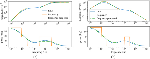
Figure 2. Weight functions for assessing a magnetic flux density (a). Weight functions for assessing an induced electric field (b). In both cases the blue curve applies in time domain, the orange curve applies in the frequency domain and the green-dashed curve is related to the proposed modification of the WPM in frequency domain. Limits for occupational exposure proposed by the ICNIRP are considered for all weight functions.
Download figure:
Standard image High-resolution image3. Analysis of standard waveforms
In this section, standard waveforms that can represent external and/or internal fields are considered. Each waveform is defined by means of specific parameters whose influence on the exposure index is evaluated through the methodology explained in section 2.1 and section 2.2. The first waveform is the trapezoidal pulse shown in figure 3(a), the second waveform is the exponential pulse shown in figure 3(b), the third waveform is the sinusoidal burst shown in figure 3(c) and the fourth waveform is the double rectangular pulse shown in figure 3(d). Each waveform has its own parameters represented in the related figure, moreover, a full description of all parameters is given in table 1.
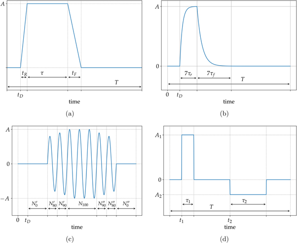
Figure 3. Standard waveforms: trapezoidal pulse (a), exponential pulse (b), sinusoidal burst (c) and double pulse (d).
Download figure:
Standard image High-resolution imageTable 1. Parameters list for each standard waveform.
| trapezoidal | A: | peak value |
| pulse | t D : | delay |
| t R : | rise time | |
| τ: | duration | |
| t F : | fall time | |
| T: | period | |
| exponential | A: | peak value |
| pulse | t D : | delay |
| τ r : | rise time constant (rise time is set to 7τr ) | |
| τ f : | fall time constant (fall time is set to 7τf ) | |
| T: | period | |
| sinusoidal | f: | fundamental frequency |
| burst | A: | peak value |
| tD : | delay | |
| Nx : | number of complete cycles with amplitude at x % of the peak | |
| double | t1: | start time of the positive pulse |
| pulse | τ1: | duration of the positive pulse |
| rectangular | A1: | positive peak |
| t2: | start time of the negative pulse | |
| τ2: | duration of the negative pulse | |
| A2: | negative peak, set to  to impose zero mean value to impose zero mean value | |
In this paper the waveforms from figures 3(a) to (c) are used to represent an external magnetic flux density, whereas the waveform in figure 3(d) is used to represent an induced electric field. Due to Faraday's law of induction, an induced quantity in the human body has a mean value equal to zero. Therefore, in this study the parameter A2 is not independent of the other parameters and it is defined as  to force a zero mean value.
Before starting with the UQ analysis it is instructive to apply the WPM in time domain, frequency domain and with the proposed modification in frequency domain (in legends and tables summarized with frequency proposed) to the standard waveforms. For the sake of shortness, only the results for the trapezoidal pulse and the double pulse are presented. The parameters used for the trapezoidal pulse are: tD = 100 ms, tR = 5 ms, τ = 300 ms, tF = 10 ms, T = 1 s. The peak of the waveform is selected to have EI=1 for the WPM in time domain. Considering the ICNIRP 2010 reference levels for occupational exposure, the waveform is processed with the weight function of figure 2(a). Figure 4(a) represents the weighted pulse for the three methods, i.e. the argument inside curly brackets in equation (7). In the legend the exposure index EI (i.e. the peak of the waveform) is shown. It is well known that the weight function of the WPM applied to a magnetic flux density is similar to a high-pass filter (Jokela 2000, ICNIRP 2003), this is confirmed by the fact that the maximum exposure is registered close to the maximum time derivative of the signal (during the rise time). The waveform related to the WPM in time domain varies smoothly as the one related to the proposed method in frequency domain. On the contrary, the standard WPM in frequency domain is characterized by several oscillations caused by the sharp variations of the phase in the weight function. Considering the WPM in time domain as the reference (i.e. EI = 1), the standard method in frequency domain underestimates the peak by 9% and the proposed approach overestimates the peak by 16%. More details will be given later in the UQ analysis about this aspect.
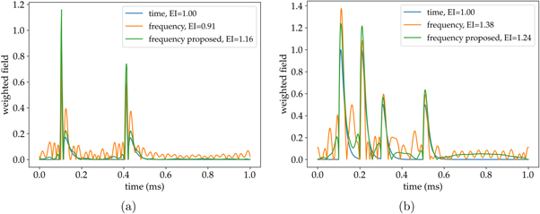
Figure 4. Application of the WPM to a trapezoidal pulse (a) and to a double pulse (b). In both cases the plot represents the weighted waveforms (i.e. the argument inside curly brackets in equation (7)) obtained with the three methods. The legend includes the value of the exposure index EI, that is the peak of each curve.
Download figure:
Standard image High-resolution imageRegarding the double pulse, the parameters used are t1 = 100 ms, τ1 = 100 ms, τ2 = 300 ms, T = 1 s. The peak A1 is selected to have EI = 1 for the WPM in time domain. The peak A2 is computed to have zero mean value as explained earlier. Considering the ICNIRP 2010 basic restrictions for occupational exposure, the waveform is processed with the weight function of figure 2(b). Looking at the results of figure 4(b) similar considerations to the case of the pulse can be done with the exception that the filter behavior, in this case, is similar to a low-pass filter (Jokela 2000, ICNIRP 2003, 2010). Regarding the exposure index provided in the legend, the standard method and the proposed method in frequency domain overestimates the values of EI by 38% and 24%, respectively. However, once again, the aspect of more interest for the aim of this paper is that the proposed approach in frequency domain remove all the oscillations in the weighted waveform.
3.1. Sensitivity analysis
The analysis presented in this section starts from two qualitative considerations. The first one is about Faraday's law. It is well known that in the low frequency range the induced currents in the human body are not strong enough to modify the applied external magnetic field (Dawson and Stuchly 1996), therefore, it is straightforward to conclude that the maximum value of the induced electric field is proportional to the maximum time derivative of the magnetic flux density ( ). The second consideration is related to the basic mechanisms of electrostimulation, that is, if we consider a rectangular pulse of induced electric field, for a given duration of the pulse, the impact is higher for a higher peak value (Reilly et al
1985).
). The second consideration is related to the basic mechanisms of electrostimulation, that is, if we consider a rectangular pulse of induced electric field, for a given duration of the pulse, the impact is higher for a higher peak value (Reilly et al
1985).
Exploiting these qualitative considerations, this section presents a sensitivity analysis of the WPM in time domain and in frequency domain (both standard and proposed). For each standard waveform two parameters are selected with these criteria: the first parameter must be strongly related to the exposure index and the second one, on the opposite, must be weakly related to the exposure index. Sobol' sensitivity indices are then computed with the aim to verify if the method used provides results in agreement with the basilar mechanisms of electromagnetic induction and electrostimulation recalled above.
In the sensitivity analysis the trapezoidal pulse, the exponential pulse and the sinusoidal burst are considered as a magnetic flux density with a given peak value. Therefore, in these cases, the parameter with strongest/weakest influence on the exposure index is the one with strongest/weakest correlation with the maximum time derivative of the waveform. The double pulse is instead assimilated to an induced electric field with a given duration. Therefore, the parameter with strongest/weakest influence on the exposure index is the one with strongest/weakest correlation with the peak value. In the list below, for each standard waveform, it is possible to read complete information about meaning of the waveform, the weight function considered in the WPM, the value of fixed parameters, the strongly and weakly parameter related to the exposure index selected for the sensitivity analysis. For the two parameters used in the sensitivity analysis, it is always considered a normal distribution with mean value equal to the one summarized in the list below and a standard deviation equal to 1% of the mean value. Furthermore, preliminary simulations have been carried out by varying the polynomial order (Spina et al 2012, Zhang et al 2013). It is found a stability of the results for polynomial order above 11. For this reason, in this paper the order of the polynomial in the PCE method is set to 12. Finally, the fixed parameters are selected to stress the methods as much as possible. For instance, in the case of the sinusoidal burst, the fundamental frequency is set to 300 Hz that corresponds to a real zero of the weight function and, consequently, to a sharp variation of the phase for the standard WPM in frequency domain. Similar considerations have been done to define the fixed parameters for the other waveforms.
- Trapezoidal pulse:
- meaning: magnetic flux density
- weight function: reference levels for occupational exposure (see figure 2(a))
- fixed parameters: tD = 100 ms, tF = 10 ms, T = 1 s, A = 1000 μT
- strongly related parameter: tR = 2 ms
- weakly related parameter: τ = 300 ms
- Exponential pulse:
- meaning: magnetic flux density
- weight function: reference levels for occupational exposure (see figure 2(a))
- fixed parameters: tD = 10 ms, T = 1 s, A = 1000 μT
- strongly related parameter: τR = 10 ms
- weakly related parameter: τF = 25 ms
- Sinusoidal burst:
- meaning: magnetic flux density
- weight function: reference levels for occupational exposure (see figure 2(a))
- fixed parameters: A = 1000 μT and 11 cycles corresponding to
 , , , , N90'' = 1, N80'' = 1, N0'' = 2
 - strongly related parameter: frequency f = 300 Hz
- weakly related parameter: tD set to half of the fundamental frequency (≈1.66 ms)
- Double pulse:
- meaning: induced electric field
- weight function: basic resurrections related to the central nervous system for occupational exposure (see figure 2(b))
- fixed parameters: t1 = 100 ms, τ1 = 50 ms, τ2 = 80 ms, T = 1 s
- strongly related parameter: A1 = 0.1 V/m
- weakly related parameter: t2 = 500 ms


The results of the sensitivity analysis are summarized in table 2. The first column describes the waveform and the two parameters used in the sensitivity analysis. The first parameter listed is the one that, according to the qualitative considerations, should be more closely related to the value of the exposure index. The second column recalls the meaning of the waveform and the limit used to build the weight function. The rest of the table provides the values of the Sobol' indices where: S1 is related to the first parameter, S2 to the second parameter and S12 to the combination of them.
Table 2. Results of the sensitivity analysis. Sobol' indices, expressed as percentages, for the standard waveforms.
| waveforms | filter | Sobol' | time | freq. | freq. |
|---|---|---|---|---|---|
| (parameters) | type | index (%) | proposed | ||
| trapezoidal | B-field | S1 | 94.505 | 10.054 | 85.062 |
| pulse | (occupational) | S2 | 1.948 | 89.924 | 7.676 |
| (tR , τ) | S12 | 3.548 | 0.022 | 7.263 | |
| exponential | B-field | S1 | 100.000 | 78.666 | 99.985 |
| pulse | (occupational) | S2 | 0.000 | 21.186 | 0.015 |
| (τr , τf ) | S12 | 0.000 | 0.148 | 0.00 | |
| sinusoidal | B-field | S1 | 100.000 | 95.001 | 99.994 |
| burst | (occupational) | S2 | 0.000 | 2.381 | 0.002 |
| (f, tD ) | S12 | 0.000 | 2.618 | 0.004 | |
| double | E-field | S1 | 100.000 | 71.284 | 99.971 |
| pulse | (occupational) | S2 | 0.000 | 28.713 | 0.029 |
| (A, t2) | S12 | 0.000 | 0.003 | 0.000 | |
The WPM in time domain is compliant with the qualitative consideration for all waveforms In fact, as shown in the 4th column, S1 is always the index with the highest value. The same does not happen in the 5th column that refers to the standard WPM in frequency domain. In fact, the value of S2 is always higher than expected with a very misleading results obtained for the trapezoidal pulse because S2 is even higher than S1. In the 6th column the Sobol' indices are provided for the proposed modification of the WPM in frequency domain. It is apparent that, by means of the correction proposed for the phase of the weight function, the method provides Sobol' indices that are in agreement with the qualitative considerations.
It is worth noting that, one should not expect to have identical results for the three methods because, even if they start from the same definition, the implementation is different. Therefore, for a given parameter, they can be more of less sensitive. But for all the methods one should expect a behavior compliant with the basilar mechanisms of electromagnetic induction and electrostimulation. Bearing this in mind, one can conclude that the sharp variations in the phase of the weight function defined in the frequency domain can compromise the sensitivity to some parameters. This issue can be avoided with a simple correction of the phase definition.
3.2. Parametric analysis
In the previous section, for each waveform, two parameters have been selected according to qualitative considerations. The sensitivity analysis confirmed them providing also quantitative information by means of Sobol' indices. In this section, more details about the behavior of the WPM in time and frequency domain is given by means of a parametric analysis. The parameter weakly related to the exposure index is varied within a reasonable range. For each value of the parameter the PCE method is used to quantify its influence on the exposure index. A small variation of the input is imposed by considering a normal distribution with standard deviation equal to 5% of the parameter value. For the sake of shortness, only the trapezoidal pulse end the double pulse are considered. As in the previous section, the trapezoidal pulse is assimilated to a magnetic flux density and the double pulse to an induced electric field.
Results are shown in figure 5, they represent the mean value of the exposure index with its 95% confidence interval. All results are normalized by the EI obtained with the WPM in time domain (i.e. the most stable method according to the literature (Keller 2017, Schmid et al 2019)) for the first value of the parameters (e.g. EI obtained with τ = 100 ms in the case of trapezoidal pulse). Before discussing the results, it is important to stress that we are analyzing the influence of a parameter that is expected to have a low correlation with the exposure index and, therefore, a small standard deviation corresponding to a narrow confidence interval should be expected. Bearing this in mind, figure 5(a) shows the results for the trapezoidal pulse. We observe that both WPM in time domain and the proposed WPM in frequency domain provide very stable results with a 95% confidence interval that is so thin that can be hardly appreciated. The two methods provides different mean values for the exposure index mainly because the weight functions have different magnitudes as shown in figure 2. Therefore, the fact that the proposed WPM in frequency domain overestimates the exposure must not be considered as a failure, the results depends both on the definition of the weight function and the spectrum of the waveform. The more important aspect is instead that both curves allow us to conclude that the duration of the pulse τ has no influence on the exposure index, as it is expected. The same consideration does not apply to the standard WPM in frequency domain. In this case the confidence interval is high enough to be appreciated and the mean value of the exposure index is not constant over the range analyzed. For the double pulse the results are summarized in figure 5(b) and the same comments already done for the trapezoidal pulse apply.
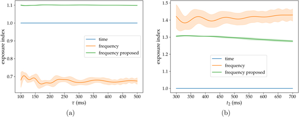
Figure 5. Parametric analysis for the trapezoidal pulse (a) and for the double pulse (b). All curves represent the mean value of the exposure index with its confidence interval. For the WPM in time domain and for the proposed WPM in frequency domain the confidence interval is so narrow that can be hardly noticed.
Download figure:
Standard image High-resolution imageQuantitative results related to the width of the confidence interval are summarized in table 3. Actually, the width of the confidence interval is expressed as a percentage of the mean value with the formula 3.92 σ/μ 100. For both waveforms it is possible to observe that the WPM in time domain exhibits a width of the confidence interval which tends to 0 % (the actual value is 3.1E − 12 % for both waveforms). This means that this method is very precise in determining that the parameter under consideration is weakly related to the value of the exposure index. On the opposite, the confidence interval for the standard WPM in frequency domain is not negligible. Finally, the proposed modification of the WPM in frequency domain reduces the width of the confidence interval significantly, more than one order of magnitude in the case of the trapezoidal pulse and approximately one order of magnitude in the case of the double pulse.
Table 3. Width of the confidence interval expressed in percentage with respect to the mean value. These data are related to figure 5.
| waveform | c.i. width | time | freq. | freq. |
|---|---|---|---|---|
| (%) | proposed | |||
| trapezoidal | average | 0.00 | 5.28 | 0.13 |
| pulse | max | 0.00 | 12.26 | 0.44 |
| double | average | 0.00 | 5.53 | 0.74 |
| pulse | max | 0.00 | 9.75 | 1.09 |
A final parametric analysis with a different aim is presented in this section. The waveform considered is the sinusoidal burst and, in this case, it is more instructive to consider the influence of the parameter strongly related to the exposure index, that is the fundamental frequency. For each value of the fundamental frequency, the peak of the sinusoidal burst (see figure 3(c) and table 1) is set to the peak magnetic flux density corresponding to the reference level proposed by the ICNIRP for occupational exposure, (i.e.  ). Results are shown in figure 6(a). It is apparent that the proposed approach in the frequency domain provides an exposure index almost constant and close to 1 with a very narrow confidence interval. This can be explained considering that, in this analysis, the peak of the sinusoidal burst is defined exactly as the inverse of the magnitude of the weight function in the frequency domain. It is worth noting that, this consideration applies also to the standard WPM in frequency domain, however, the orange curve is much more noisy than the green one. Of course, this is due to the sharp variations of the phase in the weight function. Finally, the blue curve, related to the WPM in time domain, can be explained considering figure 6(b). This plot shows the ratio between the mean values of the exposure index related to the methods in frequency domain and the one in time domain. Moreover, a third curve is introduced (with black circles). It represents the ratio of the magnitude of the weight function in frequency domain (WFf
, orange or green curve in figure 2(a)) and time domain (WFt
, blue curve in figure 2(a)). It is interesting to note that it is almost perfectly overlapped with the green curve. This means that the deviation between the proposed WPM in frequency domain and the WPM in time domain shown in figure 6(a) can be associated completely to the difference in the magnitude of the related weight functions. In fact, the phase of the weight function with the proposed modification is a very good approximation of the one in time domain as show in figure 2. The analysis of figure 6(a) together with figure 2(a) confirms also that, taking as a reference the WPM in time domain, the proposed approach overestimates the exposure index where WFf
> WFt
and it underestimates the exposure index when WFf
< WFt
. On the opposite, close to 300 Hz, the standard WPM in frequency domain overestimates the exposure index even if the WFf
≈ 0.707 WFt
.
). Results are shown in figure 6(a). It is apparent that the proposed approach in the frequency domain provides an exposure index almost constant and close to 1 with a very narrow confidence interval. This can be explained considering that, in this analysis, the peak of the sinusoidal burst is defined exactly as the inverse of the magnitude of the weight function in the frequency domain. It is worth noting that, this consideration applies also to the standard WPM in frequency domain, however, the orange curve is much more noisy than the green one. Of course, this is due to the sharp variations of the phase in the weight function. Finally, the blue curve, related to the WPM in time domain, can be explained considering figure 6(b). This plot shows the ratio between the mean values of the exposure index related to the methods in frequency domain and the one in time domain. Moreover, a third curve is introduced (with black circles). It represents the ratio of the magnitude of the weight function in frequency domain (WFf
, orange or green curve in figure 2(a)) and time domain (WFt
, blue curve in figure 2(a)). It is interesting to note that it is almost perfectly overlapped with the green curve. This means that the deviation between the proposed WPM in frequency domain and the WPM in time domain shown in figure 6(a) can be associated completely to the difference in the magnitude of the related weight functions. In fact, the phase of the weight function with the proposed modification is a very good approximation of the one in time domain as show in figure 2. The analysis of figure 6(a) together with figure 2(a) confirms also that, taking as a reference the WPM in time domain, the proposed approach overestimates the exposure index where WFf
> WFt
and it underestimates the exposure index when WFf
< WFt
. On the opposite, close to 300 Hz, the standard WPM in frequency domain overestimates the exposure index even if the WFf
≈ 0.707 WFt
.

Figure 6. Parametric analysis for the sinusoidal burst (a). Ratio of the mean value provided by the methods in frequency domain and the WPM in time domain compared with the ratio of the magnitudes of the related weight functions (b).
Download figure:
Standard image High-resolution imageIn conclusion, since the magnitudes of the weight functions in the frequency domain are identical (see figure 2), the deviation of the orange curve from the green curve shown in figure 6 can be associated to the phase definition of the standard WPM in frequency domain. For this reason, it is not a surprise that the deviation is higher close to real zeros and poles (e.g. 25 Hz, 300 Hz, and 3 kHz) where the sharp variations of the phase are localized.
4. Application of WPM to real measurements
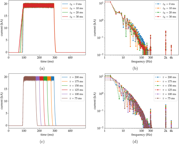
In this section the WPM is applied to several actual waveforms. A medium frequency direct current welding gun is considered as source of magnetic flux density. This device generates a pulsed field with trapezoidal shape. The waveform is not ideal because the static converter creates a ripple that is superposed to the trapezoidal pulse. The ripple has a fundamental frequency of 2 kHz and it includes higher harmonics (even up to 20 kHz) (Canova et al 2016, 2018, Giaccone et al 2020). In this paper, the current flowing in the electrodes of the welding gun is measured by varying the rise time and the weld time (i.e. the duration of the pulse called τ in figure 3(a)). Afterward, the magnetic flux density is obtained by scaling the waveform of the current to obtain the desired peak of magnetic flux density. This is possible due to the fact that, close to the electrodes, the magnetic flux density is proportional to the welding current. By means of the control panel of the welding gun the rise time value has been set to 0 ms, 10 ms, 20 ms and 30 ms. The weld time value has been set to 75 ms, 100 ms, 125 ms, 150 ms, 175 ms and 200 ms. All possible combinations have been analyzed for a total of 24 waveforms figures 7(a) and (b) show four currents with their spectrum considering different rise time values and equal weld time set to the maximum value (200 ms). Figures 7(c) and (d) show four currents with their spectrum considering different weld time values and equal rise time set to the minimum value (0 ms).
Figure 7. Measured waveforms. Welding currents with weld time equal to 200 ms and different rise time values (a) and their related spectrum (b). Welding currents with rise time equal to 0 ms and different weld time values (c) and their related spectrum (d).
Download figure:
Standard image High-resolution image
All the 24 waveforms have been scaled to have a peak of 2500 μT and tested with the three implementations of the WPM. Results are summarized in table 4. The subscript t is used for the WMP in time domain, the subscript f for the one in frequency domain and the subscript fp for the proposed modification in frequency domain. Both absolute value and normalized value of the exposure index are provided. In the case of the normalized value, the exposure index obtained with the WPM in time domain is used as the reference. Bearing this in mind, it is apparent that the results obtained processing the actual waveform confirm all the information provided in previous sections. In fact, both WPM in time domain and the proposed modification in the frequency domain provide an exposure index that is independent of the weld time and strongly dependent on the rise time. On the opposite, the standard WPM in frequency domain does not provide stable results by varying the weld time. For instance, in the case of maximum rise time (30 ms) the exposure index varies from a minimum of 0.64 to a maximum of 0.75. These values correspond to an underestimation of 2% and an overestimation of 17% with respect to the value obtained with the WPM in time domain, that is 0.65. It must be stressed again that it is not of particular importance the amount of underestimation/overestimation because it depends on the different definition of the magnitude of the weight function and also on the spectrum of the waveform considered. In this case, as shown in figures 7(b) and (d), the spectrum of the waveforms considered is very strong below 100 Hz. In this frequency range the magnitude of the weight function in frequency domain is higher that the one in time domain (see figure 2(a)). Therefore, as explained in section 3.2, it is expected an overestimation of the exposure index provided by both frequency domain implementations of the WPM. It is more important to focus on the stability/accuracy of the exposure index. The analysis on actual measurements confirms that the uncertainty budget associated to the standard WPM in frequency domain is higher than the one in time domain causing it to be sensitive to parameters that should be unrelated to the exposure index. The proposed modification to the definition of the weight function makes it possible to avoid this issue.
Table 4. Exposure index computed for all the measured waveforms The subscript t is used for the WMP in time domain, the subscript f for the one in frequency domain and the subscript fp for the proposed modification in frequency domain.
| rise time | weld time | EIt | EIf | EIfp |

|

|

|
|---|---|---|---|---|---|---|---|
| tr = 0 ms | τ = 75 ms | 1.17 | 1.27 | 1.44 | 1.00 | 1.08 | 1.23 |
| τ = 100 ms | 1.17 | 1.27 | 1.43 | 1.00 | 1.08 | 1.22 | |
| τ = 125 ms | 1.17 | 1.27 | 1.43 | 1.00 | 1.08 | 1.22 | |
| τ = 150 ms | 1.17 | 1.35 | 1.43 | 1.00 | 1.15 | 1.22 | |
| τ = 175 ms | 1.17 | 1.30 | 1.44 | 1.00 | 1.10 | 1.22 | |
| τ = 200 ms | 1.17 | 1.30 | 1.44 | 1.00 | 1.11 | 1.22 | |
| tr = 10 ms | τ = 75 ms | 0.96 | 1.08 | 1.20 | 1.00 | 1.13 | 1.25 |
| τ = 100 ms | 0.96 | 1.12 | 1.19 | 1.00 | 1.16 | 1.24 | |
| τ = 125 ms | 0.96 | 1.10 | 1.19 | 1.00 | 1.15 | 1.24 | |
| τ = 150 ms | 0.96 | 1.18 | 1.20 | 1.00 | 1.23 | 1.25 | |
| τ = 175 ms | 0.96 | 1.13 | 1.20 | 1.00 | 1.18 | 1.25 | |
| τ = 200 ms | 0.96 | 1.12 | 1.20 | 1.00 | 1.17 | 1.25 | |
| tr = 20 ms | τ = 75 ms | 0.76 | 0.77 | 0.95 | 1.00 | 1.01 | 1.25 |
| τ = 100 ms | 0.76 | 0.82 | 0.94 | 1.00 | 1.08 | 1.24 | |
| τ = 125 ms | 0.76 | 0.81 | 0.95 | 1.00 | 1.06 | 1.24 | |
| τ = 150 ms | 0.76 | 0.87 | 0.95 | 1.00 | 1.15 | 1.25 | |
| τ = 175 ms | 0.76 | 0.83 | 0.95 | 1.00 | 1.10 | 1.25 | |
| τ = 200 ms | 0.76 | 0.82 | 0.95 | 1.00 | 1.07 | 1.25 | |
| tr = 30 ms | τ = 75 ms | 0.65 | 0.64 | 0.82 | 1.00 | 0.98 | 1.26 |
| τ = 100 ms | 0.65 | 0.71 | 0.81 | 1.00 | 1.10 | 1.25 | |
| τ = 125 ms | 0.65 | 0.75 | 0.82 | 1.00 | 1.17 | 1.26 | |
| τ = 150 ms | 0.64 | 0.71 | 0.82 | 1.00 | 1.10 | 1.27 | |
| τ = 175 ms | 0.65 | 0.73 | 0.82 | 1.00 | 1.14 | 1.27 | |
| τ = 200 ms | 0.64 | 0.69 | 0.81 | 1.00 | 1.07 | 1.26 | |
5. Conclusions
In this paper the uncertainty quantification associated to the assessment of human exposure to pulsed or multi-frequency fields has been analyzed. Among all the approaches for the assessment, the weighted peak method has been selected for the analysis because it is suggested by the ICNIRP guidelines and it is also taken as a reference in other context such as the European Directive dealing with occupational exposure. The selection of a single method is not a limitation because the approach used for the uncertainty quantification is based on the polynomial chaos expansion theory and, therefore, it is very general and applicable to any method. Moreover, the tool used is a free and open source Python program (Giaccone 2018).
This paper analyzed the exposure to several standard waveforms pointing out quantitatively, through a sensitivity analysis, the parameters with more influence on the exposure index. It is shown that the WPM in time domain provide results in agreement with the basilar mechanisms of electromagnetic induction and electrostimulation. On the opposite, the WPM in frequency domain is found to be too sensitive to parameters that should not influence the exposure index. The reason of this misleading behavior is associated to the definition of the weight function in the frequency domain that has sharp variations of the phase centered on real zeros and poles. To overcome this issue, a new definition for the phase of the weight function in frequency domain is proposed. Basically, it is suggested to define the phase as it is done in classical Bode diagrams. It is shown that the proposed WPM in frequency domain is more precise than the standard one, in fact, the related sensitivity indices are closer to the ones obtained in time domain.
The output of the sensitivity analysis is used to set up a parametric analysis with the aim of evaluating the uncertainty propagation of the three methods: WPM in time domain, standard WPM in frequency domain and proposed WPM in frequency domain. For the case analyzed, it is shown that the width of the confidence interval is approximately zero for the WPM in time domain. The proposed WPM in frequency domain exhibits a so narrow confidence interval that can be hardly noticed in the presented plots. On the contrary, for the standard WPM in frequency domain, a not negligible confidence interval has been registered. A narrow confidence interval means that the mean value of the exposure index is evaluated with more precision. Therefore, it is possible to conclude that the WPM in time domain is the most precise method analyzed, the proposed modification of the WPM in frequency domain makes it possible to obtain a comparable/reasonable precision and the standard WPM in frequency domain is the less stable method.
The three methods have been also tested on measured waveforms with trapezoidal shape generated by a welding gun. Measurements have been done by varying the rise time (parameter with strong influence on the exposure index) and the weld time (parameter with weak influence on the exposure index). By increasing the rise time, all methods provide a deceasing value of the exposure index in agreement with what it is expected. By increasing the weld time (for a given rise time) results are stable only for the WPM in time domain and the proposed modification in the frequency domain. In the case of the standard WPM in frequency domain the exposure index presents a fluctuation (−2% to +17%) because, as shown in the previous analysis, this method is not as stable as the others.
In conclusion, this papers confirms that, regarding the weighted peak method, its implementation in the time domain is the more accurate and precise. Citing Keller (2017), the WPM in time domain can be used without a second thought. The standard WPM in frequency domain has some issues ascribable to how the phase of its weight function is defined. With the proposed modification of the phase definition, also the WPM in frequency domain provides performances similar to the one in time domain. In the author opinion, the proposed modification for the phase definition in frequency domain should be considered in a future revision of the ICNIRP guidelines.
Data availability statement
The data that support the findings of this study are openly available at the following URL/DOI:https://github.com/giaccone/wpm_uncertainty. Data will be available from 16 March 2023.