

Abstract
This work presents an analytical relationship between gradient-spoiled and RF-spoiled steady-state signals. The two echoes acquired in double-echo in steady-state scans are shown to lie on a line in the signal plane, where the two axes represent the amplitudes of each echo. The location along the line depends on the amount of spoiling and the diffusivity. The line terminates in a point corresponding to an RF-spoiled signal. In addition to the main contribution of demonstrating this signal relationship, we also include the secondary contribution of preliminary results from an example application of the relationship, in the form of a heuristic denoising method when both types of scans are performed. This is investigated in simulations, phantom scans, and in vivo scans. For the signal model, the main topic of this study, simulations confirmed its accuracy and explored its dependency on signal parameters and image noise. For the secondary topic of its preliminary application to reduce noise, simulations demonstrated the denoising method giving a reduction in noise-induced standard deviation of about 30%. The relative effect of the method on the signals is shown to depend on the slope of the described line, which is demonstrated to be zero at the Ernst angle. The phantom scans show a similar effect as the simulations. In vivo scans showed a slightly lower average improvement of about 28%.
Export citation and abstract BibTeX RIS
Introduction
Rapid gradient-echo sequences are a common choice for fast 3D imaging of tissues with short relaxation times (Scheffler and Lehnhardt 2003). This includes musculoskeletal (MSK) tissues such as cartilage and knee meniscus. Gradient-spoiled steady-state sequences dephase residual magnetization before the next acquisition, leading to stimulated echoes after the spoiler gradient in later repetitions. Double-echo in steady-state (DESS) collects signal echoes both before and after the spoiler (Bruder et al 1988, Lee and Cho 1988, Redpath and Jones 1988). The residual transverse magnetization can also be made completely incoherent using RF spoiling, such as in spoiled gradient recalled echo (SPGR), fast low angle shot (FLASH) or T1 fast-field echo (T1-FFE).
In MSK imaging, DESS has been found to have more sensitivity to low-rate changes in cartilage morphometry than FLASH and producing more reliable morphology measurements in the posterior femur (Eckstein et al 2006, Wirth et al 2010). The two DESS echoes can be averaged, resulting in one, high-SNR signal (Hardy et al 1996, Ruehm et al 1998). However, if the two echoes are not combined but rather used to generate separate images, their relative amplitudes can be used to obtain an estimate of T2 based on steady-state signal models (Welsch et al 2009, Heule et al 2014, Dregely et al 2016, Sveinsson et al 2017). Furthermore, altering the size of the DESS spoiler gradient enables diffusion weighted imaging and estimation of the apparent diffusion coefficient (ADC) (Bieri et al 2012a, Staroswiecki et al 2012, Sveinsson et al 2019). FLASH has been shown to have higher precision in femoropatellar cartilage and superior detection of cartilaginous and cortical bone abnormalities (Eckstein et al 2006, Algin et al 2010). One study found FLASH to provide better bone-cartilage contrast than DESS, while DESS has been shown to provide good contrast between cartilage and synovial fluid against other tissues (Hardy et al 1996, Moriya et al 2009, Friedrich et al 2011, Bieri et al 2012b). The DESS and FLASH sequences can thus complement each other well in joint imaging studies. Studies such as the osteoarthritis initiative (OAI) therefore used both DESS and FLASH for morphological knee imaging (Peterfy et al 2008).
Due to its steady-state, gradient-spoiled nature, the relationship between the DESS signals and parameters of the tissue and the pulse sequence is inherently complicated. Various DESS relationships have been derived (Wu and Buxton 1990, Freed et al 2001, Hänicke and Vogel 2003), but a simple, closed-form expression of the signal behavior would still be beneficial. Prior knowledge of different contrasts of the signals following a tractable curve could be used for gaining intuition of the signal behavior, parameter estimation (Fram et al 1987, Wang et al 1987), and model-based denoising (Jang and Hwang 2012). While several multi-contrast MRI denoising methods have been developed (Lam et al 2014, Gong et al 2015, Veraart et al 2016, Manjón and Coupé 2018, Song et al 2020), such a model-based denoising method could complement these approaches. Therefore, there is an unmet need for an intuitive, tractable signal model describing the DESS signals as a simple function of sequence and tissue parameters.
In this work, we introduce a novel and simple signal relationship between gradient-spoiled and RF-spoiled steady-state signals. After analyzing this relationship, which can be considered the main contribution of this study, as a secondary contribution we also give a preliminary demonstration of one of its several applications in the form of a heuristic denoising method of diffusion weighted DESS signals, applicable when two DESS acquisitions with separated echoes and an RF-spoiled scan such as SPGR or FLASH are acquired in the same protocol. We validate this relationship and the denoising approach in simulations, phantom scans, and in vivo scans.
Theory
Relationship between gradient- and RF-spoiled signals
A simple analytical relationship between the two DESS echoes results from the Bloch equations in combination with the steady-state condition of the magnetization being periodic over a repetition time. In the extended phase graph (EPG) matrix formalism (Hennig et al 2003, Weigel et al 2010, Weigel 2015), the magnetization M is represented by a matrix:

with (*) denoting a complex conjugate. Fn
represents the transverse magnetization dephased by n spoiler gradients, while Zn
represents the longitudinal component. The observable signal is F0. A gradient shifts the coefficients Fn
. The effects of T1/T2 decay, as well as diffusion, on state n can be described by the scaling terms ![${E}_{2,n}={e}^{-\displaystyle \frac{{\rm{TR}}}{T2}-\left[\left({n}^{2}+n+\displaystyle \frac{1}{2}\right){\rm{TR}}-\displaystyle \frac{\tau }{6}\right]{\rm{\Delta }}{k}^{2}D}$](https://content.cld.iop.org/journals/0031-9155/66/1/01NT03/revision3/pmbabce8aieqn1.gif) and
and  where Δk = γGτ, G and τ are the gradient amplitude and duration, respectively, and D is diffusivity. T1 relaxation is represented by an additive factor to Z0. The effect of an RF pulse with flip angle α and phase ϕ is represented by matrix multiplication with the matrix
We label the time points right before/after the RF pulse with −/+, respectively.
If the magnetization immediately after the RF pulse, M(0+), has the form of equation (1), then right before the next pulse (after the passage of one TR) it will have the form
Without loss of generality we can assume the RF pulse is about Mx , so ϕ = π/2, giving real Fn . Due to the steady-state condition, R(α, π/2)M(TR−) = M(0+) or, equivalently, R(−α, π/2)M(0+) = M(TR−). Comparing the transverse and longitudinal DC (leftmost) states gives


Eliminating Z0 and writing the acquired DESS signal amplitudes before and after the spoiler, respectively, as  and
and  gives
gives

This can be rearranged as follows:

Equation (5) describes a line, where the slope ψ is the term in parentheses, and the intercept β is simply the RF-spoiled signal SRF (with zero transverse magnetization before RF pulses):

In equation (5), the coefficients ψ and β are independent of diffusion (or, equivalently, independent of the spoiler gradient). The signals S1 and S2 change with diffusion, however. The signals from DESS scans with varying spoilers therefore fall on a line in the (S2, S1) coordinate system, with positions along the line dependent on spoiler moment and diffusivity. In the limit of  non-zero diffusion results in no signal at the second echo and thus S1 converges to the intercept point β = SRF. The derivation giving equation (6) assumes nothing about the signal behavior other than the Bloch equations and the steady-state condition.
Using the model as a denoising prior
A heuristic denoising method results from the described model by noting that a DESS point (S2, S1) may deviate from the line described in equation (6) due to noise. Given such noisy data points, an estimate for the line can be calculated by minimizing the sum of the squared distances of each point to the line (Fasano and Vio 1988), which can be written as

Here, H and L represent acquisitions with high and low diffusion weighting, respectively. This can be solved numerically for ψ and β using gradient descent. This is different from the ordinary least squares best fit line, which only assumes that the vertical values are noisy and thus only minimizes the vertical squared difference.
The noise of the complex signal components can be reasonably assumed to be independent, identically distributed (i.i.d.) Gaussian noise. While performing a magnitude operation on the complex data can cause a deviation from this noise behavior, it has been established that this deviation is very small except for very low levels of SNR (Gudbjartsson and Patz 1995). For SNR levels such as in this study, working with magnitude data is not expected to cause substantial deviations of this kind, but this was further investigated through our experiments.
Therefore, assuming that the noise errors in S1 and S2 are i.i.d., the maximum likelihood estimate for a point that has deviated from the theoretical line due to noise will be the closest point on the line. This estimate can be obtained by simply projecting the corrupted point to the line obtained with equation (7) in the (S2, S1) coordinate system.
Methods
We evaluated our line-based signal model and denoising method with simulations as well as phantom and in vivo scans, with parameters as shown in table 1. Spoiler gradient moments will be specified with the number of dephasing cycles (full rotational differences between spins in a voxel) produced by the gradient over a 3 mm slice, where Gn = n · 7.83 mT m−1 · ms gives n cycles of dephasing. This is a convenient unit as it should ideally be kept at integer values for proper spoiling.
Table 1. Parameters for simulations, phantom scans, and in vivo scans.
| Simulations | Phantom | In vivo | |
|---|---|---|---|
| TR (ms) | 20.0 | 20.0 | 20.0 |
| TE (ms) | 5.0 | 5.0 | 5.5 |
| α (°) | 25 | 25 | 25 |
| DESS gradient duration (ms) | 3.4 | 3.4 | 3.4 |
| DESS gradient moments (dephasing cycles over 3 mm) | 0.01, 20 | 2, 4, 7, 10, 12, 15, 18, 20 | 2, 20 |
| FOV (cm × cm × cm) | — | 20 × 20 × 12 | 20 × 20 × 12 |
| Imaging matrix | — | 256 × 256 × 40 | 384 × 320 × 40 |
| Scan time (mm:ss) | — | 7 × 2:43 | 3 × 3:25 |
All scans were performed on a 3T 750 scanner (GE Healthcare, Waukesha, WI). Informed subject consent was obtained in accordance with the Institutional Review Board protocol at our institution. All in vivo scans used a 16-channel flexible receive coil that wrapped around the knee (GEM Flex by NeoCoil). All scans used a water-selective spectral-spatial radiofrequency pulse.
Simulations
Analysis of signal model
To validate the relationship in equations (5), (6) and to estimate its sensitivity to noise and scan parameters, simulations were performed using the EPG formalism (Weigel et al 2010, Weigel 2015), including contributions from magnetization dephased by up to 6 spoiler gradients for accurate signal estimation.
First, the validity of equation (6) was tested by simulating DESS signals in the (S2, S1) coordinate system with spoiler gradient moments ranging from 2 cycles to 60 cycles. Tissue parameters of T1 = 1.2 s, T2 = 40 ms, and ADC = 1.5 μm2 ms−1, typical of cartilage, were adopted.
Then, simulations were performed to examine the relationship of equation (6) in the presence of noise. 1024 noisy instances of DESS points (S2L , S1L ) with low diffusion weighting (0.01 cycles), DESS points (S2H , S1H ) with high diffusion weighting (20 cycles), and an SPGR data point SSPGR were generated with complex gaussian noise at an SNR of 100 in the S1L signal (the S1L signal will generally be used for an SNR reference throughout this study). This was done for T2 = 30, 35, ... 65 ms and ADC = 1.3, 1.35, ... 1.65 μm2 ms−1 (T1 being kept fixed at 1.2 s), resulting in 64 tissue types, and the average result over all tissue types examined. For illustrative purposes, a subset of 10 noisy samples of each point was plotted in the (S2, S1) coordinate system for the parameters T2 = 40 ms and ADC = 1.5 μm2 ms−1. Finally, to investigate the behavior of the slope ψ in equation (6), ψ was plotted for flip angle α = 1°–90°, first with T1 = 0.8–1.5 s and T2 fixed at 40 ms, and then with T2 = 20–80 ms and T1 fixed at 1.2 s. TR/TE were kept fixed at 20/5 ms.
Investigating model as prior for denoising
Next, we investigated the effect of our proposed denoising method of projecting the noise-corrupted points to the estimated signal line by setting the final estimate as

where λ is between 0 and 1. Here, λ serves as a weight factor to explore whether a combination of the measured point and the projected point can yield better SNR than a simple projection. With λ = 0, the signal measurements are trusted completely while with λ = 1, the measurements are required to lie on the line described in equations (5), (6). The estimation performance was measured by the reduction in signal standard deviation. This was tested for a range of λ (with flip angle α = 25°) and α (with λ = 1), with SNRS1L = 100.
To investigate the dependency of the denoising method on SNR and on the effect of using magnitude or complex data, the reduction in standard deviation and the signal bias resulting from the method were also computed over a range of SNRS1L for both magnitude and complex data. This was measured for the parameters in table 1.
Phantom scans
Ten agar phantoms with T2 in the range of 45–65 ms were simultaneously scanned and a sample slice was examined. The validity of the model was investigated by examining data points from several gradient moments, as described in table 1. The effect of denoising, which only used 2 DESS gradient moments of 2 cycles and 20 cycles, as well as an SPGR scan, was measured by calculating the reduction in the standard deviation of an ROI drawn inside each phantom with λ = 1. Denoising was done voxel by voxel, with the line calculated and the denoising performed separately for each voxel coordinate. While this will lead to a variation in the line slopes due to the noise in each voxel, this was not expected to lead to an average error in the line estimation as all data points were considered to have independent, identically distributed unbiased noise, as was investigated in simulations. The measured standard deviation was modeled as the sum of noise variation (σ N ) and real variation in the agar(σ R ):

The direct measurement of the relative reduction in total signal variation will only act as a lower bound of the reduction of signal variation from noise. To get a better estimate of the noise-free signal variation, the 20-cycle scan was performed with 10 scan repetitions, which reduces σ N by a factor of √10:

Applying equations (9), (10) to both the 1-repetition scan and the 10-repetition scan, in combination with equation (6), gives an estimate for σ N . Then, the relative noise improvement from the projection procedure was measured by computing Δσmeasured/σ N .
In vivo scans
Sagittal scans were performed on the knee of a healthy volunteer. The scans consisted of DESS with spoiler gradients giving 2 and 20 cycles of spoiling, and an RF spoiled SPGR scan (parameters in table 1). The reduction in signal standard deviation was measured after applying the denoising method (λ = 1) to a sample slice. As for the phantoms, the method described in equations (9), (10) was used, but this time the higher-SNR reference only used 3 repetitions to keep scan times reasonable for the subject. For comparison with a commonly used denoising method, the denoising results in a low-SNR tibial ROI were compared with those obtained with 3 × 3 Wiener filtering (Fan et al 2019).
Results
Simulations
Analysis of signal model
The simulation results for gradients ranging from 2 to 60 cycles are shown in figure 1(a). The simulations confirm that the noiseless measurements lie on a line with the largest signal values corresponding to the smallest gradient moment. The line terminates at the S1 axis at the RF-spoiled signal, giving the same signal as a theoretical spoiler gradient with infinite moment. Figure 1(b) shows the 10 noisy samples with T2 = 40 ms and ADC = 1.5 μm2 ms−1, illustrating how the signals deviate from the theoretical line in the presence of noise. Figures 1(c), (d), showing ψ as a function of α, T1, and T2, demonstrate that the slope becomes largely independent of α and T1 at higher values of α, but does not lose sensitivity to T2. The simulations show the slope becoming zero at the Ernst angle, and negative for smaller flip angles.

Figure 1. Model simulation results. (a) DESS signals, plotted in the (S2, S1) plane, simulated over a range of spoiler gradient moments. The signals form a line as described in equations (5), (6). The numbers show the spoiler gradient moment in dephasing cycles over a 3 mm slice. (b) Simulations of DESS scans with low spoiling and weak diffusion weighting (blue), high spoiling and strong diffusion weighting (green), and an RF-spoiled scan (red). Noise was added to several instances of the simulations. The results demonstrate how noise causes the data to deviate from the line-forming relationship in equations (5), (6). The denoising method of this study involves producing a more accurate estimate of the signals by projecting them to this line. (c) The slope ψ in equation (6) over a range of flip angles α and T1, with T2 fixed at 40 ms. Note that ψ becomes close to constant after about α = 30°. (d) ψ over a range of α and T2, with T1 fixed at 1.2 s. For all T2 values, the slope becomes zero at the Ernst angle, which can also be observed in panel (c).
Download figure:
Standard image High-resolution imageInvestigating the model as prior for denoising
Figure 2(a) demonstrates that a larger value of λ generally improves the estimate, with the best results at λ = 1, where the signals are made to lie on the closest point on the line. This was the setting used for all subsequent processing. The improvement is most apparent in the signal S1H , comparable to a doubling in scan time.
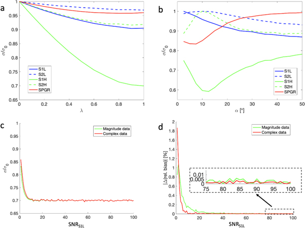
Figure 2. (a) The resulting reduction in signal standard deviation by partial or full projection of the measured data to the line in panels (a), (b). The parameter λ signifies how much the signal gets projected, as shown in equation (8). (b) The reduction in signal standard deviation for varying flip angles and λ = 1. The S1H signal experiences the greatest denoising at the Ernst angle, where the line in figures 1(a), (b) is flat. The baseline signal at this angle is smaller, however, so this study employed a flip angle of 25°. (c) Comparison of standard deviation reduction of S1H when using magnitude or complex data, keeping α = 25°. The effect is very similar for moderately high SNR. (d) The resulting introduction of bias when using magnitude or complex data, measured as a percentage of the true signal. The magnitude data starts exhibiting bias at higher levels than the complex data, but for normal ranges of SNRS1L , bias is negligible (inset). Note that the plot shows absolute value and the introduced bias in the complex data was negative.
Download figure:
Standard image High-resolution imageFigure 2(b) shows the reduction in standard deviation of each signal for different values of the flip angle α. The improvement in S1H
is largest (40% reduction) at the Ernst angle,  However, at the same flip angle, no improvement is seen in S2H
and S2L
as the slope there is zero, giving no information about S2.
However, at the same flip angle, no improvement is seen in S2H
and S2L
as the slope there is zero, giving no information about S2.
Figure 2(c) demonstrates very similar reduction in standard deviation whether magnitude data or complex data is used. Figure 2(d) shows that for both data types, the estimate increases signal bias when SNR is very low. However, at SNR levels expected in clinical scans, shown in the figure inset, using magnitude data produces no appreciable bias.
Phantom scans
The phantom signal values, averaged over a sample region of interest (ROI), follow the predicted line very closely. Figure 3(a) demonstrates this in three sample phantoms (no. 1, 8, and 10 in figure 3(b)). The reduction in total standard deviation, after applying the method on the 2- and 20-cycle DESS scans and the SPGR scan, was on average about 20% (figure 3(b)). This can be viewed as a floor to the actual noise reduction, since the total standard deviation includes variation from signal as well as noise. The reduction relative to the estimated noise standard deviation was about 35%, in agreement with the simulation results in figure 2. On average, the mean signal change was −0.3% (with standard deviation 0.1%).

Figure 3. Results from phantom scans. (a) By varying the spoiler gradient moment, the measured signals form a line in (S2, S1) space, terminating in the RF-spoiled signal, as described in equations (5), (6) and simulated in figure 1(a). The plots shows 3 sample phantoms, numbered 1 (red), 8 (blue), and 10 (green) in panel b. (b) The signal standard deviation in an ROI of each phantom after applying the denoising procedure in equation (8) with λ = 1, relative to the standard deviation before denoising. The blue bars show the relative change in total standard deviation, while the red bars show the relative change in standard deviation due to noise, estimated as shown in equations (9), (10). The results are in good agreement with the expected average reduction of 30% in figures 2(a), (b).
Download figure:
Standard image High-resolution imageFigures 4(b), (c) show a zoomed-in version of the ROI outlined in figure 4(a) (and shown in green in figure 3(a)), before and after the denoising procedure, demonstrating a more uniform ROI after denoising. Figures 4(d), (e) show a histogram of the pixels in figures 4(b), (c). The standard deviation is reduced by about 28%, with the ROI mean changing by about −0.4% (other phantoms showed even less change).
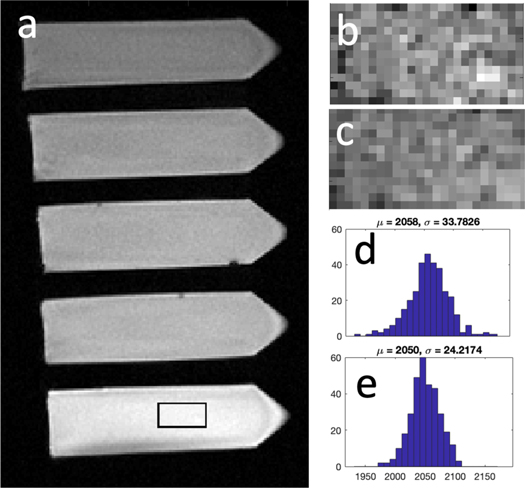
Figure 4. Closer analysis of the phantom data in figure 2. In a sample slice, ROIs were drawn in each of the 10 phantoms scanned. Panels (b), (c) show zoomed-in versions of the ROI shown in panel (a), before and after the denoising procedure described. Visually, the ROI looks less noisy, and this is further demonstrated in panels (d), (e), which show the histogram of the pixels within the ROI before and after denoising. The standard deviation decreases by about 28%, while the mean value of the ROI changes only marginally.
Download figure:
Standard image High-resolution imageIn vivo scans
The results from the in vivo scans are shown in figure 5. The reduction in noise-induced SNR was estimated to be 32%, 29%, and 24% for the tibial, femoral, and patellar cartilage, respectively. The comparison of images before and after denoising of the tibial cartilage (figures 5(b) and (c), respectively) indicates that the denoising process leads to better agreement with the higher-SNR scan (figure 5(d)). The difference in performance for the denoising algorithm suggests a possible dependency on the SNR level of the tissue being examined, as the tibia, femur, and patella had SNR levels of 80, 120, and 150, respectively, but this could also be due to artifacts such as motion or parameter differences.

Figure 5. In vivo results. Panel (a) shows a sagittal slice of the first DESS echo. The smaller panels focus on the tibial region in the small rectangle. Panels (b), (c) show the tibial cartilage before and after the denoising procedure, respectively, in the ROI drawn in panel (a). The denoising procedure makes the cartilage more closely resemble a less noisy, 3-repetition scan shown in panel (d). Regions that are abnormally dark (yellow arrow) in panel (b) are less pronounced in panel (c), compared to panel (d). The absolute difference between panels (b) and (d) is shown in panel (e), while that between panels (c) and (d) is shown in panel (f). Panel (g) shows the denoising effect in different cartilage regions.
Download figure:
Standard image High-resolution imageFigure 6 shows the comparison of the 3-repetition scan to the results from the denoising method presented in this study and to the results from 3 × 3 Wiener filtering of the image. Clearly, the line-based method (figure 6(b)) retains several image details that are smoothed out by the Wiener filter (figure 6(c)). At the same time, the numerical performance in a tibial ROI was better for the line-based method than for the Wiener filtering, both in terms of the estimated reduction in noise-induced standard deviation (32% versus 23%, respectively), and the reduction in total absolute pixel intensity difference compared to the 3-repetition scan (34% versus 10%, respectively).

Figure 6. Comparison of the baseline 3-repetition image of the tibial cartilage (a) to results from the line-based denoising method presented (b) and to the results from 3 × 3 Wiener filtering (c).
Download figure:
Standard image High-resolution image
Discussion
We have presented a model describing the DESS data points with different spoiler gradients forming a line in the signal coordinate system, terminating in the RF-spoiled signal value. Our model can be used as a constraint for the signal measurements, as shown in the heuristic denoising method presented. The method is applicable when a DESS scan with weak diffusion weighting and an RF-spoiled scan are acquired under the same scan settings, making use of shared signal information between such scans. This could involve a quantitative joint examination protocol, including FLASH and a weakly diffusion-weighted DESS scans for bone, cartilage, and soft tissue morphology and two DESS scans for T2 and diffusion estimation.
Much modeling has been done of gradient-spoiled signals (Wu and Buxton 1990, Freed et al 2001), but such models have often either involved theoretical approximations or resulted in non-closed-form expressions, less suitable for intuitive signal analysis and more difficult to incorporate into image processing methods. The presented model is simple and yet involves no approximations as it is only based on the steady-state condition and the Bloch equations. This sole dependency on first-principle steady-state MR physics provides a very strong prior.
In phantoms, the estimated reduction in signal standard deviation from noise agreed well with simulations. Less denoising was achieved in vivo, possibly due to motion as the method assumes no motion between scans so that scan and tissue parameters remain the same for a given voxel between all three scans. It should be noted that the predicted 30% improvement in the highly diffusion weighted image does not outperform averaging two repeated scans. Therefore, the denoising approach has its primary use for protocols already including all three scans, where it can be run without extra cost in scan time. It is also important to note that the presented denoising approach does not preclude the use of other denoising methods, which can be run jointly with the method shown here.
The heuristic denoising approach presented in this work is only one of many potential applications of the model shown in equations (5), (6). Other uses include image synthesis (e.g. using S1H , S1L , S2L , and SRF to synthesize the S2H signal, which can often suffer from image artifacts) or parameter estimation (e.g. measuring the slope of the line and then estimating the either the flip angle α, the longitudinal relaxation T1, or the transverse relaxation T2, assuming two of these parameters are known). Figures 1(c), (d) show that sensitivity to deviations in flip angle is high near the Ernst angle, where the line becomes flat. At high flip angles, sensitivity to T1 and α is low while sensitivity to T2 is high. Therefore, flip angle estimations could be done by imaging at the Ernst angle, while T2 estimations could be done at higher flip angles. Comparing this type of flip angle estimation to existing methods, such as the Bloch–Siegert approach (Sacolick et al 2010), is an interesting future direction of this work. Additionally, the model provides intuition for the behavior of gradient-spoiled and RF-spoiled signals under different scan settings.
Many methods exist for signal denoising, with some major approaches using common methods such as filtering or regularization (Fan et al 2019) while others enforce a general prior, such as edge correlation or patch similarity, in multi-contrast studies (Bilgic et al 2011, Manjón et al 2012, Haldar et al 2013, Lam et al 2014, Song et al 2020). Our approach has the benefit of relying on an analytical signal model of spoiled steady-state sequences based on first-principle steady-state MR physics. Therefore, it does not involve trade-offs between SNR and resolution and can be jointly used with other methods.
The model presented is robust towards imperfections in B0 and B1. As the signals are spoiled, their amplitude is not affected by constant B0 inhomogeneities over a voxel, assuming the spoiling is done effectively. A linear B0 imperfection term over a voxel would lead to intra-voxel dispersion that will act as a change in T2', but the line relationship will still hold. The model will therefore hold for first-order B0 imperfections. The effect of B1 deviations would be to change the value of the flip angle α equally for all the sequences. The line relationship would still hold, simply with a different value of α. As demonstrated in figures 1(c), (d), this would lead to a change in the slope of the line, and a difference in denoising performance as demonstrated in figure 2(b), but for expected deviations in B1, these effects should not be substantial.
This study includes some limitations. Although the presented method should work on any MSK tissue, only healthy cartilage was examined. Future studies could investigate other tissues such as the meniscus, muscle, or diseased cartilage. Also, only one in vivo subject was scanned as described in this proof-of-concept study. Furthermore, the effects of the presented method on the mapping of quantitative parameters such as T2 and the ADC were not examined. This could be explored by applying previously described DESS quantification methods and comparing to results obtained with gold standard methods (Saritas et al 2008). Additionally, the derivation of equation (5) did not account for eddy currents, which would affect the two echoes differently and possibly cause deviations from the linear relationship. No such effects were observed in our experiments, but future work could involve simulating such deviations as a function of gradient ramping. Another interesting future direction could be to perform the estimation of the line (equation (7)) using L1 minimization. This could make the line estimate less sensitive to noisy data points, at the cost of a more complex implementation. Our method assumes that relaxation parameters and flip angle are constant within a voxel, which is reasonable for high-resolution scans. While T2* in cartilage, the MSK tissue focused on in this work, is likely at least biexponential, our scans are likely not sensitive enough for the shorter relaxation components to have an appreciable effect on our signals. Other MSK tissues, such as muscle, would likely also not have a detectable short-T2* component in conventional scans, although this could become detectable in ultra-short echo time imaging. Lastly, it should be noted that the main contribution of this note is the signal model in equations (5), (6) and its value as a prior for various image processing approaches. The analysis of the denoising application is therefore limited and it can be regarded as a preliminary demonstration of one of many potential applications, for which a more complete analysis could be done in a follow-up study. Figures 3(b) and 5(g) show a performance variability between image regions, and variability was also noted between data sets, as another knee data set (not shown), acquired with a lower resolution, saw a lower noise reduction performance of 11%–15%. A separate study could analyze whether this is due to differences in tissue characteristics, B1 inhomogeneities, motion, or in the assumptions behind equations (9), (10), which may not hold well in practice for small ROIs. This could involve acquiring maps of tissue parameters and B1, applying motion correction, and instead of using equations (9), (10) for estimating performance, repeating the scans several times and examining the statistical distribution of the outcomes with and without the denoising applied. While outside the scope of this note, such a study presents an interesting future direction of this work.
In conclusion, we have presented a relationship between gradient- and RF-spoiled steady-state signals and shown it can be used as a prior for constraining signal measurements when collecting both gradient-spoiled DESS scans and RF-spoiled scans such as FLASH or SPGR.