
Abstract
Proton computed tomography (pCT) has high accuracy and dose efficiency in producing spatial maps of the relative stopping power (RSP) required for treatment planning in proton therapy. With fluence-modulated pCT (FMpCT), prescribed noise distributions can be achieved, which allows to decrease imaging dose by employing object-specific dynamically modulated fluence during the acquisition.
For FMpCT acquisitions we divide the image into region-of-interest (ROI) and non-ROI volumes. In proton therapy, the ROI volume would encompass all treatment beams. An optimization algorithm then calculates dynamically modulated fluence that achieves low prescribed noise inside the ROI and high prescribed noise elsewhere. It also produces a planned noise distribution, which is the expected noise map for that fluence, as calculated with a Monte Carlo simulation. The optimized fluence can be achieved by acquiring pCT images with grids of intensity modulated pencil beams. In this work, we interfaced the control system of a clinical proton beam line to deliver the optimized fluence. Using three phantoms we acquired images with uniform fluence, with a constant noise prescription, and with an FMpCT task. Image noise distributions as well as fluence maps were compared to the corresponding planned distributions as well as to the prescription. Furthermore, we propose a correction method that removes image artifacts stemming from the acquisition with pencil beams having a spatially varying energy distribution that is not seen in clinical operation. RSP accuracy of FMpCT scans was compared to uniform scans and was found to be comparable to standard pCT scans.
While we identified technical improvements for future experimental acquisitions, in particular related to an unexpected pencil beam size reduction and a misalignment of the fluence pattern, agreement with the planned noise was satisfactory and we conclude that FMpCT optimized for specific image noise prescriptions is experimentally feasible.
Export citation and abstract BibTeX RIS

Original content from this work may be used under the terms of the Creative Commons Attribution 3.0 license. Any further distribution of this work must maintain attribution to the author(s) and the title of the work, journal citation and DOI.
1. Introduction
Radiotherapy using protons allows to precisely deliver the planned dose to the tumor while minimizing radiation exposure of critical structures outside of the treatment beam path. Proton therapy, therefore, is believed to have better outcome with less severe side effects compared to conventional radiotherapy using x-rays for certain anatomical sites (Weber et al 2012, Park et al 2015, Nakajima et al 2017). During treatment, protons stop inside the tumor, where, just before stopping, their energy loss spikes within the so-called Bragg peak. While this allows to achieve sharp dose gradients and to spare healthy tissues, proton therapy is sensitive to range uncertainties (Paganetti 2012) and thus requires frequent and accurate imaging (Engelsman et al 2013, Landry and Hua 2018). The current clinical practice for acquiring spatial maps of the stopping power relative to water (RSP) of the patient is to employ x-ray computed tomography (CT) images and to apply a calibration converting interaction of photons with matter (attenuation) to interaction of protons with matter (RSP). This yields range errors of up to 3% (Yang et al 2012), which need to be considered with additional dose margins and conservative beam directions, and necessarily increase the dose to healthy tissue.
To avoid conversion errors, RSP maps can directly be acquired using proton CT (pCT) as originally proposed by Cormack (1963) and later experimentally realized by Hanson et al (1978). A pCT scanner measures the residual energy of protons after traversing the patient or an object (for a review of contemporary pCT scanners see Johnson (2018)). Since protons gradually lose energy, and given that the initial proton energy is known, the energy loss is directly linked to a water-equivalent path length (WEPL), that is the path length in water, in which a proton would lose the same amount of energy. For a proton crossing an object, the WEPL is a line integral through the RSP along the curved path of the proton in the same way that the logarithmic intensity is a line integral through the attenuation coefficient for x-ray CT. Unlike in x-ray CT, however, line integrals are not along straight lines and spatial resolution can suffer severely if not accounted for correctly (Krah et al 2018). Therefore, pCT scanners typically also measure proton positions and directions prior and after the patient allowing to estimate the proton's trajectory and incorporating it in the reconstruction algorithm (Li et al 2006, Rit et al 2013, Hansen et al 2016). A recent study by Dedes et al (2019) comparing the accuracy of state-of-the-art dual-energy x-ray CT to the performance of a prototype pCT scanner concluded that errors are on par between the two modalities and suggested that artifact reduction may considerably improve the pCT performance.
Besides having good RSP accuracy, pCT images may potentially be acquired at very low imaging doses of only 1 − 2 mGy per tomography (Hansen et al 2014, Meyer et al 2019) based on an estimate using a homogeneous phantom (Schulte et al 2005). Dickmann et al (2019) showed increased noise levels due to the heterogeneity in an anthropomorphic phantom suggesting that imaging doses may range from 2 mGy to 6 mGy for the same noise level in heterogeneous phantoms. A low imaging dose is especially important for particle therapy, where the delivery of the treatment is divided in up to 30 fractions and changes in positioning of the patient or movement of internal organs must be tracked by imaging as frequently as possible to ensure a safe delivery of the therapeutic dose (Landry and Hua 2018). However, imaging for online adaptation only requires knowledge about the RSP within the limited sub-volume covered by the treatment beams. To exploit this, we recently developed an algorithm for dose reduction with fluence-modulated pCT (FMpCT), an imaging technique adapted from Bartolac et al (2011) to pCT by Dedes et al (2017). The optimization method (Dickmann et al 2020) tries to achieve an inhomogeneous image noise prescription using dynamically modulated fluence fields. Modulation is achieved by pCT acquisition using a grid of pencil beams. The output of the optimization algorithm are relative weights for pencil beams within every projection of the tomography. Using a Monte Carlo simulation, a corresponding 'planned noise distribution' can be calculated, which is the noise map expected for the optimized set of pencil beam weights. The Monte Carlo code models the geometry of an existing prototype pCT scanner (Giacometti et al 2017) and realistic pencil beams at a clinical facility (Dickmann et al 2020). It was also validated for fidelity in terms of image noise (Dickmann et al 2019) and RSP accuracy (Giacometti et al 2017, Dedes et al 2019). We prescribed low image noise (high image quality) within the volume covered by typical treatment beam configurations, which we label the region-of-interest (ROI), and high image noise (low image quality) elsewhere. This resulted in a considerable dose saving outside of the ROI by up to 40%, which depends on the phantom and shape of the ROI. The dose saving was shown to be superior to the simpler intersection approach used by Dedes et al (2019). However, since the noise-planning study employed the same Monte Carlo code as was used to generate data input to the optimizer, an experimental validation was indispensable.
The aim of this work, therefore, was to experimentally validate and reproduce the computational results obtained by Dickmann et al (2020). We employed the same fluence patterns and used the same three phantoms that were modeled there. To employ modulated fluence patterns, we interfaced the control system of a pencil beam scanning (PBS) beamline at the Northwestern Medicine Chicago proton center and obtained tomographies using the preclinical phase II pCT scanner (Johnson et al 2016, Bashkirov et al 2016). We evaluated our ability to accurately control image noise by comparing experimental image noise maps to the corresponding planned noise as well as to the prescription. In the process, we identified image artifacts stemming from the pencil beam acquisitions and operation of the beamline in research mode and removed them successfully with a correction method. Finally, we tested the accuracy of RSP values by comparing mean values and distributions inside and outside of the ROI.
2. Materials and methods
2.1. Experimental setup
Data for this work was acquired using the phase II pCT scanner developed by Johnson et al (2016) and Bashkirov et al (2016). As depicted in figure 1, the scanner consists of two tracking modules, one prior and one after the phantom, and a scintillating energy detector. Protons emitted from the PBS beamline are individually registered by four silicon strip detectors in each of the two tracking modules, resulting in coordinate measurement pairs prior and after the phantom. The tracking system maintains a detection efficiency above 99% at trigger rates up to 1 MHz for the entire field-of-view and is capable of recovering missed hits if at least three of the four position measurements are available (Johnson et al 2016). It has also been shown to safely sustain hit efficiency at 400 kHz under increased local count rates when operating with pencil beams (Dedes et al 2018). The two coordinate measurement pairs allow for an estimation of the proton's direction vector before and after the object, which helps to determine a most likely path through the object (Schulte et al 2008). Eventually, the proton's residual energy is measured using a five-stage scintillating energy detector. Because the mean initial energy of the protons is known and they gradually lose energy when traversing the object, the residual energy measurement can be used to calculate the WEPL along the proton's path. This uses a calibration curve generated with an object of known geometry and RSP (Piersimoni et al 2017). To allow for tomographic data acquisition, the phantom is mounted on a rotation stage.
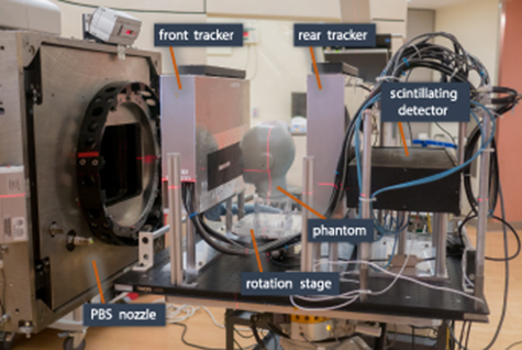
Figure 1. The phase II pCT scanner installed on a robotic arm at the Northwestern Medicine Chicago proton center. The important components of the scanner are indicated as well as the pencil beam scanning (PBS) nozzle.
Download figure:
Standard image High-resolution image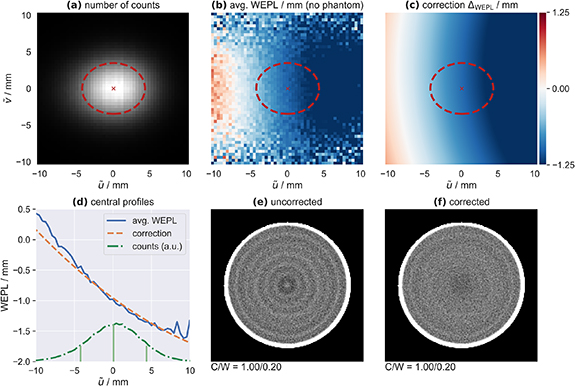
Figure 2. Illustration of the effect of the pencil beam WEPL correction: (a) number of counts over all registered pencil beams, (b) the average uncorrected WEPL, (c) the optimized correction function, (d) profile plots for (a) to (c) along  for
for  (counts are in arbitrary units on the secondary axis), (e) an uncorrected RSP reconstruction and (f) the corrected reconstruction. (a) to (d) are given in coordinates
  relative to the pencil beam center. In (a) to (d) the expectation value and the FWHM ellipse is indicated (for (d) as a projection to the
  -axis). (b) and (c) share the same color scale.
Download figure:
Standard image High-resolution imageThe scanner is located at the Northwestern Medicine Chicago proton center, a clinical facility for proton therapy equipped with a beamline (PROTEUS PLUS, Ion Beam Applications SA, Louvain-la-Neuve, Belgium) with full PBS capability. Delivery of the proton fluence using pencil beams was a key requirement for this study, as it allowed employing individually modulated proton fluence fields. While the scanner is typically operated using a broad beam, data acquisition using PBS and static fluence fields has been shown to be feasible by Dedes et al (2018) using protons and Volz et al (2018) using helium ions (at another facility).
2.2. Image reconstruction and noise for proton CT
Data output from the scanner is in so-called 'list-mode.' Thus, for every registered proton, this list includes five quantities: position and direction vector prior to the object and subsequent to it as well as the WEPL inferred from the energy measurement. To obtain a three-dimensional map of the RSP from this data, WEPL information was binned to pixelated projections and averaged within each pixel. Prior to binning, data cuts were applied, removing protons with direction or WEPL information outside of a three standard deviation interval in each pixel of the projection, which is a common procedure in proton imaging (Schulte et al 2005, Rit et al 2013). The standard deviation in each pixel was calculated from the difference between the 30.85th percentile value and the median, which corresponds to a 0.5-standard-deviation interval and is less sensitive to the non-Gaussian tails of the distribution. Data cuts eliminated about 25% of recorded protons in air and 15% inside a homogeneous phantom. Protons were predominantly rejected due to overestimated WEPL information caused by spurious signals in the energy detector. A three-dimensional volume could be reconstructed using a special cone-beam filtered backprojection algorithm (Rit et al 2013) making use of the most likely path information and thereby improving the spatial resolution in the image.
This study investigated the uncertainty of RSP values, i.e. image noise or image variance. This quantity could be calculated directly from the list-mode data by estimating the Gaussian variance of the WEPL values within each pixel of the projection and using variance reconstruction (Wunderlich and Noo 2008, Rädler et al 2018). Projection noise and hence also image noise for pCT is predominantly affected by the incident proton fluence, i.e. the number of protons contributing to the mean WEPL value in one pixel of the projection. Therefore, modulation of the incident fluence was the principal lever for adjusting image noise. However, to carefully predict the absolute level of image noise in pCT for a given fluence level, various contributions had to be taken into account. A previous study by Dickmann et al (2019) identified (1) the incident energy spread output from the accelerator, (2) energy straggling inside the object and (3) inside the detector, as well as (4) multiple Coulomb scattering, to be the main causes of image noise for pCT. In particular, multiple Coulomb scattering was found to strongly depend on the object's heterogeneity. Consequently, prior knowledge of the object's geometry is required to precisely predict the image noise level at a given incident fluence using a validated Monte Carlo simulation such as in Dickmann et al (2019).
2.3. Fluence optimization algorithm
FMpCT may be performed by employing a regularly spaced set of pencil beams and individually modulating the fluence of each pencil beam resulting in inhomogeneous image noise distributions as originally shown by Dedes et al (2017) and Dedes et al (2018). To prescribe arbitrary image noise distributions, we employed the optimization algorithm of Dickmann et al (2020), which requires an object model to calculate individual pencil beam weights. The algorithm consists of three steps, which are briefly summarized here and can be studied in detail in the original publication:
- (a)For a given phantom geometry, use a Monte Carlo simulation to predict variance levels in the projection for unit fluence (i.e. all relative weights set to unity).
- (b)Use an iterative method to calculate a stack of variance projections that yield the prescribed image noise map (thus transfer the problem from image space to projection space).
- (c)Calculate the required relative fluence as the ratio of the two variance quantities taking into account a non-linear inverse relationship between fluence and variance. Then, fit a pencil beam model to the required fluence to get relative pencil beam weights.
The algorithm thus outputs relative pencil beam weights resulting in a planned noise distribution, which can be calculated to check the agreement with the initial noise prescription by employing the optimized pencil beam weights in a Monte Carlo simulation. Note that the planned noise was the best achievable noise distribution by our optimization algorithm and could differ from the prescription. Moreover, the optimizer tried to achieve peak noise equal to the prescription in the ROI and thus average noise may be below the prescription.
2.4. Phantoms
We used three phantoms in this study: a cylindrical water phantom, an anthropomorphic head phantom and a sensitometry phantom. The water phantom consisted of a cylindrical container made from polystyrene and was filled with distilled water. The head phantom (ATOM , Model 715 HN, CIRS Inc., Norfolk, USA) mimicks the head of a 5 year old child using tissue-equivalent materials. The sensitometry phantom was the cylindrical CTP404 module of the Catphan
 600 phantom (Phantom Laboratory, New York, USA) and features several inserts of different materials. To obtain the planned noise distributions and fluence patterns, phantom models were used in the Monte Carlo simulation by Dickmann et al (2020), and details can be found therein. RSP values of the phantoms were characterized experimentally in other studies (Dedes et al 2019, Giacometti et al 2017) and are also matched in the Monte Carlo engine by adjusting the mean excitation energy.
2.5. Noise prescriptions and pencil beam grids
We aimed at achieving the following image acquisitions: (1) unit fluence with all relative pencil beam weights set to one, which corresponded to the standard acquisition with PBS in pCT and served as a comparison, (2) a prescription of constant image noise  throughout the phantom, which was shown to reduce dose at equal peak-noise level, and (3) a ROI imaging task with a prescribed variance
  inside one quadrant of the image (i.e. the ROI; corresponding to a potential two-beam treatment configuration in proton therapy), and a higher prescribed variance
  outside the ROI, which allowed for dose reduction. In all evaluations we labeled the three cases (1) unit, (2) constant, and (3) FMpCT. The value of
  was chosen to be the peak variance of the unit fluence acquisition and thus depended on the phantom (Dickmann et al 2019). For the water phantom this was
  , for the head phantom
  and for the sensitometry phantom
  . A graphical representation of the FMpCT ROI is included in figures 3, 4, 6. Note that the ROI corresponded to prescription A in Dickmann et al (2020), which yielded imaging dose savings of 40% and 39% outside the ROI for the water and head phantoms, respectively.
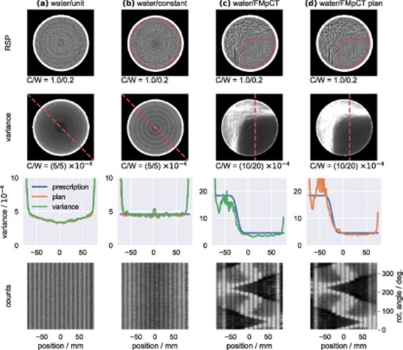
Figure 3. Proton CT acquisitions for the water phantom: (a) unit fluence scan, (b) constant noise prescriptions and (c) FMpCT scan together with (d) the planned noise distribution for the FMpCT scan. The four rows display: the reconstructed RSP maps, the corresponding variance maps, profiles through the variance maps, the prescription and the corresponding planned noise, and counts sinograms. The ROI for the noise prescriptions is indicated by a dashed line in the RSP maps. Center (C) and window (W) settings for displaying maps are given below each map. For the counts sinograms this was C/W = 140/280 protons.
Download figure:
Standard image High-resolution image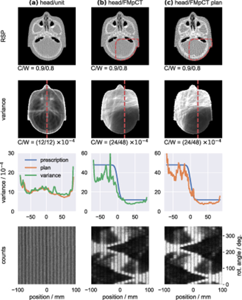
Figure 4. Proton CT acquisitions for the head phantom: (a) unit fluence scan and (b) FMpCT scan together with (c) the planned noise distribution for the FMpCT scan. The four rows display: the reconstructed RSP maps, the corresponding variance maps, profiles through the variance maps, the prescription and the corresponding planned noise, and counts sinograms. The ROI for the noise prescriptions is indicated by a dashed line in the RSP maps. Center (C) and window (W) settings for displaying maps are given below each map. For the counts sinograms this was C/W = 140/280 protons.
Download figure:
Standard image High-resolution imageThe arrangement of the pencil beam grids was also chosen in agreement with the computational planning study. From an evaluation of experimental data, Dickmann et al (2020) obtained an elliptical shape of the pencil beam with a full width at half maximum (FWHM) of  in the horizontal u-direction and
  in the vertical v direction (the rotation axis was oriented along v). Pencil beams were interspaced by
  in u and by
  in v. This corresponded to approximately
  in u and
  in v. In u the spacing was effectively also
  , because we used a quarter pencil beam shift: the whole pencil beam grid was offset in u by
  . This compensated for the larger interspace in this direction, as pencil beam patterns at 0° and 180° by were thus offset
  with respect to each other, resulting in a smooth total fluence despite the larger interspace. This is analogous to the quarter detector pixel shift used to increase the sampling rate in x-ray CT. Note that such a quarter pencil beam shift could only be performed in the u direction, and that it depends on a precise alignment of the pencil beams with respect to the coordinate system of the scanner.
2.6. Interfacing the PBS beam line
We interfaced the control system of the PBS beam line at the proton center to deliver the optimized fluence plans, in order to experimentally validate that noise maps achieved with pencil beam weights output from the optimization algorithm yield the planned noise maps and are close to the prescribed image noise maps. This required transforming the pencil beam grid description (center coordinates and relative weights) to machine instructions. The fluence was modulated by changing the dwell time of each pencil beam spot, as in Dedes et al (2018), and keeping the current constant at 1.3 nA. The instructions for the accelerator were thus set points for the scanning magnets as well as absolute dwell times. A program developed specifically for this study then converted those set points to currents applied to the scanning magnets, which required proprietary beam line information.
The maximum dwell time (the one corresponding to a relative weight of one) was chosen such that approximately four times (4 ×) the required number of protons was registered and the correct number of protons (1 ×) was selected in post-processing. In a first step, we acquired data at unit fluence without any phantom. From this data we later extracted the average number of hits within a central region of the front tracker. The same number was generated using data from the Monte Carlo simulation (with 1 × fluence) and the acceptance ratio  between experiment and simulation was calculated. For all subsequent scans, we then randomly accepted protons with a probability equal to
  , which was constant for all projections of all acquisitions, and rejected all other protons. Although the exact number of protons could have been delivered by fine tuning the maximum dwell time or the beam current on the spot, we opted for this conservative approach considering the limited available beam time.
To ensure that the pencil beam patterns were delivered in synchrony with the scanner rotation, the phantom was rotated at fixed time intervals large enough to allow for a manual initiation of each pencil beam pattern, which led to considerably longer scanning times than the 6 to  that are typically needed for scans with this prototype pCT scanner when the beam is continuously on.
2.7. Image noise evaluation
We acquired unit fluence as well as FMpCT data for the water phantom and the head phantom. For the water phantom, a constant noise fluence modulation was additionally acquired. All acquisitions were performed on the same day, except for the unit fluence acquisition of the water phantom, which was acquired on a separate day. RSP and variance maps were calculated from the acquired data. All reconstruction parameters were chosen as in Dickmann et al (2020). Image variance maps were compared to the planned noise distribution, as well as to the prescriptions. To illustrate the fluence patterns, we calculated so-called 'counts sinograms' that display the number of protons (after data cuts) contributing to the calculation of the mean WEPL in each pixel of the detector and for each rotation angle.
2.8. RSP evaluation
To verify that the FMpCT acquisition does not compromise the RSP accuracy of pCT inside the ROI, we performed two scans with the sensitometry phantom: one with unit fluence and one with the FMpCT noise prescription. Inserts of the phantom as well as the phantom body were masked and distributions of RSP values inside the masks were analyzed and compared between the fluence-modulated and the uniform fluence scan. In agreement with Dedes et al (2019), the mask of an insert was chosen to be a cylinder with a radius of  , which is half of the radius of the insert. The phantom's body is made from epoxy and inserts consist of polymethylpentene (PMP), low–density polyethylene (LDPE), polystyrene, acrylic, Delrin and Teflon, for which water-column RSP measurements can be found in Dedes et al (2019). The ROI of the FMpCT scan encompassed the PMP and the Teflon inserts which have the lowest and highest RSP values, respectively. We chose to investigate these inserts with the largest expected RSP error (Dedes et al 2019) so that this evaluation can serve as a conservative upper limit estimate and because only two inserts could be accommodated in the ROI due to the geometry of the phantom.
2.9. Pencil beam WEPL correction
In retrospective analysis of the acquired data, RSP ringing artifacts were observed which we assumed to stem from a spatially varying incident energy distribution within each pencil beam of the grid, and which were more severe than the calibration artifacts discussed in Dedes et al (2019). The distribution was assumed to be similar for all pencil beams. Since incident energy is not measured by the pCT scanner but instead assumed to be 200 MeV, a spatially varying distribution will distort the image.
To isolate this effect, we used a scan without phantom for which on average we expected a WEPL of  after data post processing. In a first step, we calculated the count rate over time and separated individual pencil beams at the drop in count rate between two spots. For each pencil beam p we then calculated the center of mass coordinate
  at the second tracking plane of the front tracker module. For each proton, the coordinates
  relative to the center of mass of the corresponding pencil beam p (again at the second plane of the front tracker) were determined. We then fitted a quadratic correction function

where a, bu, bv, cu were cv are free fitting parameters. The fitting parameters were found by minimizing the cost function
where the sum is over all N protons from all pencil beams, and  is the coordinate of proton n relative to the center of mass of its pencil beam, and wn its measured WEPL value.
To correct data of a subsequent phantom scan using equation (1), all pencil beams in the dataset needed to be separated and center of mass coordinates calculated for each of them. Then, a proton with WEPL w belonging to pencil beam p and with relative coordinates  was assumed to instead have a WEPL of
  .
.
We performed reconstructions of the constant noise prescription for the water phantom both with and without pencil beam correction to show its effect on the data. To further illustrate the pencil beam spot and its energy distribution, we binned all protons that were used to find the correction function to a grid in relative coordinates  and calculated the number of counts relative to the pencil beam center as well as their mean WEPL. From the binned counts distribution we also calculated the FWHM in both directions, which we refer to as
  and
and  .
.
2.10. Fluence sums
Since the acquisition with the quarter-shifted pencil beam grid described in section 2.5 depends strongly on a precise delivery of the fluence and misalignments could cause distortions of the resulting fluence patterns, we investigated if fluence was delivered as intended in the planning study by calculating 'fluence sums': for every proton we estimated a most likely path  based on the tracking information, where u and v are the lateral coordinates and d is the (signed) distance from the isocenter plane. For every projection n acquired at angle αn we then calculated a three-dimensional counts map Cn(u, v, d) which counts the number of most likely paths intersecting each voxel. The fluence sums F(x, y, z) were then calculated as the sum over all Cn, where each Cn was rotated along the v-axis according to its rotation angle αn and thus

where N is the number of projections. Fluence sums were calculated both for the experimental data and for the corresponding planning Monte Carlo data.
To investigate the robustness to changes of the spot size and the alignment of the fluence pattern, we performed an additional Monte Carlo planning study using the pencil beam  and
and  determined in section 2.9 instead of
  and
and  used during optimization and noted in section 2.5. We added an artificial shift su in the u-direction to this data by calculating the fluence sums with the modified equation

Fluence sums were calculated for five misalignments between  and
and  .
.
3. Results
3.1. Pencil beam WEPL correction
Figure 2(a) shows the counts distribution summed over all pencil beams in coordinates relative to the pencil beam center. The expectation value (marked with a cross) is in the center as expected. The shape of the pencil beam is not isotropic: the FWHM, indicated by a dashed line, is elliptical and wider in the  -direction. The FWHM was
  in the
  -direction and
  in the
  -direction, which is slightly smaller than
  in the
  -direction in the Monte Carlo planning study and considerably smaller than
  in the
  -direction.
Figure 2 (b) and (c) displays the average WEPL and the fitted correction function  . The correction function described the WEPL distribution well, especially within the indicated FWHM ellipse. There was a clear dependency of the WEPL distribution in the
  -direction. The dependency in the
  -direction was weaker, but still captured by the fit of the correction function. The parameters of the correction function were determined as
  ,
,  ,
,  ,
,  , and
, and  .
.
In figure 2 (d) profiles through counts, average WEPL and the correction along  and for
  are shown. In the center of the pencil beam a negative WEPL of around
  was observed. Again, there was a good agreement between the fit and the averaged WEPL, in particular for the center of the beam spot. The expectation value and the
  interval for the counts distribution are indicated by solid lines under the distribution, which was slightly left-skewed: the mode was shifted to the right but the expectation value was at
  as desired.
In figure 2 (e) and (f) two reconstructions of the water phantom for the constant noise prescription are displayed with and without the pencil beam correction. Rings in the image were efficiently removed by the correction. Minor rings and a dip in the center of the phantom remained. The average value over the whole water region ( ) changed slightly from 0.990 ± 0.024 (without correction) to 0.993 ± 0.023 (with correction).
All further reconstructions employed the pencil beam correction.
3.2. Image noise evaluation
Before reconstruction, we randomly accepted  of the measured protons after determining the actual delivered number of protons in a single run without phantom. This value is reasonable considering that we planned to acquire four times the required data (see section 2.6).
Figure 3 displays experimental results for the water phantom in (a) to (c) together with Monte Carlo results from the planning study in (d). The first row displays RSP maps for all acquisitions. The ROI for the FMpCT noise prescription is indicated by a dashed line in the RSP maps. For the constant noise prescription, this ROI was the entire phantom volume, except for the edges. In (c) and (d) a clear modulation of the noise pattern is already visible in the RSP image.
The variance map in the second row of figure 3 for unit fluence (a) showed the expected reduction in the center and an increase with increasing radius, peaking at the edges. In comparison to that the constant noise prescription in (b) was visibly more uniform, but rings distorted the flatness. Those rings could later be linked to the smaller spot size described before, together with a slight misalignment of the fluence pattern. The variance map in (c) confirmed what is already visible in the corresponding RSP map: noise for the FMpCT acquisition was low inside the ROI and high elsewhere. The planned noise in (d) was similar to the achieved noise in (c) inside the ROI, but slightly higher outside. Faint variance rings were also visible in the low variance area.
The third row displays line profiles through the variance maps as indicated by the dashed lines in the second row. Moreover, profiles through the prescription for (b) to (d) are displayed and the planned noise is added in (b) for comparison. Inside the ROI, the achieved experimental variance in (b) and (c) was in agreement with the planned noise. The prescription was achieved, considering that the optimizer tried to achieve peak variance or lower inside the ROI. In the center of (b) and outside of the ROI in (c) the experimental variance differed slightly from the prescription. However, also the planned noise in (d) differed from the prescription in this region.
The last row of figure 3 displays counts sinograms. Data is shown only for the same slice that is displayed in the first and second rows. Sinograms were not changing with the rotation angle for the unit fluence acquisition in (a). Nevertheless, the single pencil beam contributions were visible. The constant noise prescription in (b) featured reduced fluence in the center of the phantom which increased towards the edges. The counts sinograms for the FMpCT noise prescription in (c) and (d) agreed between simulation and experiment.
Figure 4 shows the same evaluations for the head phantom, albeit only for unit fluence and the FMpCT noise prescription. For unit fluence in (a) the variance map in the second row featured increased noise levels around strong heterogeneities (e.g. the nasal cavities) and the edges, as expected from previous studies. Additionally, variance rings were also noticeable, which were not expected from the simulation study (shown only as profile) and were caused by the smaller pencil beam size in combination with a misalignment as described before. The strongest variance peaks were also visible for the FMpCT noise prescription in (b), but in particular inside the ROI the variance distribution was flat as intended. Variance profiles in the third row indicate agreement of the experimental data with the planned noise (c). Both the achieved noise and the planned noise were below the prescription as the optimizer tried to achieve peak variance inside the ROI.
3.3. Fluence sums
In figure 5 (a) and (b) fluence sums are displayed (a) for all cases of the experimental study and (b) for the corresponding planning study. On the left of each column, one slice of the fluence sum, is shown and on the right of each column a perpendicular view is shown calculated along the dashed line indicated in the first panel. In general, the fluence sums of experiment and planning study showed similar modulations. Differences were caused by the smaller pencil beam size in the experimental data as well as by a slight misalignment of the grids. This was most noticeable in the perpendicular view where the single pencil beam contributions were visible in the experimental data, but were smeared out in the planning study which assumed a larger pencil beam spot size. This predominantly affected the direct vicinity of the rotation axis, which is in the center of the perpendicular view. The water/unit acquisition in (a) had constant fluence in the  -direction and just a slight drop of the summed fluence close to the rotation axis. Modulations due to the pencil beam size were visible in the z-direction. The two other water phantom acquisitions and the head/unit data in (a) showed distinct pencil beam spots both in the
  and z-direction and in particular suffered from a distinct drop of fluence in the center, which hints that the fluence patterns were slightly misaligned in these scans and that the exact quarter pencil beam shift partially failed. In contrast to that, the head/FMpCT data in (a) also showed pencil beam patterns in both directions, but exhibited an increase of the summed fluence close to the rotation axis, which suggests that a misalignment happened in the opposite direction. All experimental acquisitions, except for water/unit consequently showed rings in the summed fluence in the xy-plane, and most prominently in the center of the volume.

Figure 5. Fluence sums for (a) all experimental acquisitions of the water and head phantom and (b) for the corresponding Monte Carlo data. In (c) Monte Carlo data for the water phantom at unit fluence with the smaller spot size of the experimental data and different shifts su of the fluence pattern are shown. The three-dimensional fluence volume is displayed for one slice (showing the x and y coordinates) and as a perpendicular view along the indicated dashed line (showing the z coordinate together with a linear combination of the x and y coordinate, here indicated as  ). The color scale used for all displays is indicated with the last panel. An interactive version of this figure can be viewed in the supplementary material, available online at stacks.iop.org/PMB/65/195001/mmedia.
Download figure:
Standard image High-resolution image
Figure 6. (a) Unit fluence scan and (b) FMpCT noise prescription for the sensitometry phantom together with (c) materials of the inserts and the ROI. (d) Histograms of the RSP value distributions inside the inserts and the body for both reconstructions. (PMP: polymethylpentene, LDPE: low-density polyethylene).
Download figure:
Standard image High-resolution image
The effects of the smaller pencil beam size ( ,
,  ) and a misalignment in the fluence pattern were further investigated in simulations in figure 5(c). The simulated fluence sum with a shift of
  showed a very similar pattern as the water/unit data in (a). As the shift gets larger towards
  , an interference pattern occurs in the
  -direction as well as a prominent drop of fluence in the center. With positive values of su the fluence increased in the center.
3.4. RSP evaluation
Figure 6 displays two scans of the sensitometry phantom: one with unit fluence (a) and one with the FMpCT noise prescription (b). As indicated in (c) the Delrin, acrylic, polystyrene and LDPE inserts were outside of the ROI and were imaged with high variance—the PMP and Teflon inserts were inside the ROI and were imaged with low variance.
In figure 6(d) histograms are shown for the RSP distributions inside the inserts of the phantom as well as for the phantom body. For each insert, both the histogram of the unit fluence data and that of the fluence-modulated data are shown. Data were separated according to ROI-membership and the body was partially inside and partially outside the ROI. For the inserts outside of the ROI the distributions of the FMpCT scan were considerably broader compared to the unit fluence distributions. For the inserts inside the ROI, RSP distributions had a similar spread for the unit fluence scan and the FMpCT scan, which is expected as the variance prescription inside the ROI was equal to the peak variance in the unit fluence scan. The body exhibited only a slight broadening of its RSP distribution. There was no visible shift of the mean value of any of the distributions.
This was analyzed in detail in table 1 where for all inserts the water-column RSP value (Dedes et al 2019) is given as well as relative errors for four datasets: data with and without pencil beam energy correction as well as for unit fluence and for the FMpCT noise prescription. Uncertainties are given as the error of the mean over all voxels inside the masked volume, thus yielding smaller uncertainties for the larger body mask. We calculated the mean absolute percentage error (MAPE) from the absolute value of the relative deviation of the measured and expected RSP for each of these datasets once averaging over all inserts (MAPE-ALL) and once averaging only over the two inserts inside the ROI of the FMpCT prescription (MAPE-ROI). Corresponding standard errors were calculated by error propagation.
Table 1. RSP values and errors for all inserts and the body of the sensitometry phantom for unit fluence and the FMpCT noise prescription. Scans with and without the pencil beam corrections were analyzed. For comparison, the last column shows results from Dedes et al (2019) using the same phantom. The mean absolute percentage error is calculated from the absolute relative deviation of the measured and expected RSP values for the two inserts inside the ROI (MAPE-ROI) as well as for all inserts (MAPE-ALL). Uncertainties are given as the standard error of the mean over all voxels inside the masked volume and calculated by error propagation for MAPE-ALL and MAPE-ROI. (PMP: polymethylpentene, LDPE: low-density polyethylene).
| uncorrected error in % | corrected error in % | error in % | ||||
|---|---|---|---|---|---|---|
| Insert | RSP | unit | FMpCT | unit | FMpCT | Dedes (2019) |
| inside ROI | ||||||
| PMP | 0.883 | 0.18 ± 0.31 | 0.79 ± 0.36 | 0.51 ± 0.31 | 1.06 ± 0.35 | 1.08 ± 0.11 |
| Teflon | 1.790 | −1.31 ± 0.18 | −1.49 ± 0.21 | −1.16 ± 0.17 | −1.32 ± 0.21 | −1.31 ± 0.05 |
| outside ROI | ||||||
| LDPE | 0.979 | −0.33 ± 0.32 | 0.24 ± 0.64 | −0.12 ± 0.31 | 0.52 ± 0.65 | −0.49 ± 0.11 |
| polystyrene | 1.024 | −0.12 ± 0.30 | −0.25 ± 0.66 | 0.06 ± 0.29 | −0.11 ± 0.67 | −0.04 ± 0.10 |
| body/epoxy | 1.144 | −1.39 ± 0.02 | −1.66 ± 0.03 | −1.20 ± 0.02 | −1.54 ± 0.03 | — |
| acrylic | 1.160 | −0.80 ± 0.27 | −0.80 ± 0.57 | −0.54 ± 0.27 | −0.63 ± 0.57 | −0.30 ± 0.07 |
| Delrin | 1.359 | −0.93 ± 0.21 | −1.02 ± 0.45 | −0.78 ± 0.21 | −0.83 ± 0.45 | −1.32 ± 0.21 |
| MAPE-ALL | 0.72 ± 0.09 | 0.89 ± 0.18 | 0.63 ± 0.09 | 0.86 ± 0.18 | 0.76 ± 0.05 | |
| MAPE-ROI | 0.74 ± 0.18 | 1.14 ± 0.21 | 0.84 ± 0.18 | 1.19 ± 0.21 | 1.20 ± 0.06 | |
In the unit fluence data, RSP errors improved for all inserts, except for the PMP insert, when applying the pencil beam energy correction. The corresponding change of the MAPE-ALL, however, was less than its standard error. For the FMpCT acquisition, the MAPE-ROI of inserts inside the ROI was slightly increased by the correction, but the change was only a fraction of the corresponding standard error. Here in particular, the PMP (in the ROI) and LDPE (outside the ROI) inserts were degraded and all others improved. Changes in all inserts between corrected and uncorrected data were overlapping within the standard error of the mean, except for the body (compare distributions in figure 6 (d)). In the FMpCT scan using the correction, the MAPE-ROI was elevated compared to the corresponding unit fluence acquisition. Both inserts inside the ROI are slightly above 1% error, which is consistent with Dedes et al (2019): the error there was 1.08% for PMP (corrected FMpCT: 1.06%) and −1.31% for Teflon (corrected FMpCT: −1.32%). For a further comparison, results from Dedes et al (2019) are listed in the last column of table 1. In particular the MAPE-ALL and the MAPE-ROI agree between the two studies. Thus, the accuracy achieved in this study is comparable to Dedes et al (2019) and consequently competitive to state-of-the-art clinical dual-energy x-ray CT.
4. Discussion
4.1. Pencil beam WEPL correction
In retrospective analysis of the acquired data we identified a possible incident spatial distribution of proton energy as the cause of RSP ringing artifacts in the reconstructed images seen in figure 2(e). Such an energy distribution is not expected for the clinical treatment mode but may arise from the operation in research mode and reduction of the output fluence by closing slits in the beam line. Analysis of the proton data after transforming to coordinates relative to each pencil beam center allowed to isolate this energy spread (which manifested in a non-zero WEPL distribution in a scan without phantom). Fitting of this WEPL distribution and a subsequent subtraction allowed to flatten the WEPL distribution and to efficiently remove RSP rings in all acquisitions. Remaining rings and distortions visible in the water phantom scan are caused by inaccuracies in the detector calibration and known to distort pCT imaging accuracy (Dedes et al 2019). While previous FMpCT publications (Dedes et al 2018) also employed pencil beam scanning for static fluence modulation, their absolute noise levels were higher compared to this study which partially masked the RSP ringing artifacts. Further analysis based on de-noising confirmed that similar distortions were also present in their data.
Analysis of the pencil beam spot revealed an elliptical shape, which was expected from previous investigations (Dickmann et al 2020). However, the spot size was smaller than expected in both directions. In particular in the  -direction the spot size was almost halved. Operation of the scanner at very low proton fluence requires closing the momentum and divergence slits of the accelerator to values beyond what is commissioned for clinical use. Even though slit positions and magnet settings were equal as when estimating beam parameters in Dickmann et al (2020), it is likely that maintenance of the beam line that was performed in between the acquisitions caused this change, although the ultimate cause could not be identified. For clinical operation such a change was not observed. While we investigate the impact of the distorted fluence delivery using Monte Carlo simulations in the next section, it was not possible to repeat the the experimental study with an amended optimization as this did not seem justified given the overall successful fluence modulation observed in this data. In general, if taken into account correctly, a smaller pencil beam size may be beneficial for the fluence optimization as more subtle modulations and smaller ROIs can be achieved. However, we re-optimized the fluence for the smaller pencil beam size and the impact on the large ROI chosen in this study was small.
Correcting for a shift in the incident energy distribution may have a minor impact on noise in the image. However, it is important to note that noise was originally distorted by the shifted WEPL values and the pencil beam correction brings it back to the original, expected value. Correction is therefore mandatory and we expect a better agreement with simulations (which do not contain the pencil beam effect) after correction.
4.2. Fluence sums
Analysis of the fluence sums and comparison of the experimental data to Monte Carlo data from the planning study revealed the effect of the smaller pencil beam spot size, in particular in the z-direction, which corresponds to the  -direction of the spot size. While the simulation study, which was performed with a larger spot size, employed smooth modulation patterns, the experimental scans exhibited the pencil beam spot structure. All scans suffered from the smaller spot size in the z-direction (across the slices). Hence, in variance maps, we also expect an equivalent modulation of noise values across the slices.
One scan had a mostly smooth distribution within the slice (xy-plane). The other scans suffered from an additional misalignment of the quarter-shifted pencil beam pattern, which was characterized by a considerably reduced or, in one case, increased fluence close to the rotation axis, as well as a further unintended circular fluence pattern within the slice. This effect occurred in addition to the smaller spot size. The water/unit acquisition appears to have a better alignment than subsequent acquisitions. This is possible since it was performed on a different day. The alignment also may have changed within the magnitude of a millimeter while exchanging phantoms. We could show, using simulations, that misalignments of the order of  may introduce variance rings. Nevertheless, the variance modulations of the FMpCT prescription are much larger than the distortions caused by the pencil beam spot size and the misalignment of the pattern. Therefore, the general FMpCT prescription was still achieved.
Dose savings were not investigated in this experimental study. However, the agreement of the fluence justifies the assumptions that experimental dose savings will be comparable to those evaluated in the planning study, which were up to 40% outside of the ROI for the FMpCT noise prescription. We therefore believe that this method will help to considerably reduce imaging dose for future pCT acquisitions.
4.3. Image noise and RSP evaluation
After correcting for the pencil beam WEPL distortion, the experimental scans using two phantoms and three fluence patterns (unit fluence, constant and FMpCT noise prescription) showed a very good agreement to what was expected from the planned noise distribution. Distortions from the prescription were limited to regions outside of the ROI where also the plan did not yield the prescription. This was because the optimizer tried to achieve a peak variance equal to the prescription and remaining spikes in the planned noise distribution forced the mean variance to be lower than the prescription. Consequently, also the out-of-ROI variance was below the prescription, as the variance contrast between high-noise and low-noise region is limited as discussed in Dickmann et al (2020). In particular, for the constant noise prescription, which showed a very flat planned variance distribution, rings slightly distorted the variance map in the experimental data. These rings were not related to the pencil beam WEPL correction, but could be explained by the smaller pencil beam spot size and a slight misalignment of the patterns as described in the previous section. Nevertheless, agreement with the simulation study and with the prescription was satisfactory and the experimental realization of FMpCT was successful.
Evaluation of RSP values in a sensitometry phantom confirmed that the RSP accuracy was only slightly affected by the FMpCT acquisition and that the spread of the distribution of RSP values increased outside of the ROI but remained constant inside the ROI. While we observed slight degradations of RSP accuracy in some inserts, changes were mostly within the standard error of the mean (see table 1). RSP errors for unit fluence PBS scans agreed with values reported by Dedes et al (2019) with the same phantom and a broad beam. We therefore conclude that the PBS acquisition is feasible and does not deteriorate the pCT accuracy if the pencil beam correction is applied. An investigation of the RSP accuracy in the FMpCT prescription for the two inserts inside the ROI with the most extreme RSP values led to a slight degradation due to FMpCT which was still within the standard error of the mean. It is important to note that the FMpCT ROI on purpose covered the two inserts which also showed the largest errors in Dedes et al (2019), where the authors suggest that RSP errors are related to the design of this prototype scanner and could be avoided in a future scanner. Additionally, the FMpCT RSP errors for the inserts inside the ROI were very similar to those reported in Dedes et al (2019). In the absence of artifacts using an idealized Monte Carlo simulation, Dedes et al (2017) found no degradation of RSP accuracy with even stronger fluence modulations than those used in this study. In the data presented in this study, all observed measurement errors were of the order of magnitude expected for a typical pCT scan. We, therefore, conclude that FMpCT can reduce dose (and increase noise) outside of a ROI while maintaining the required accuracy inside the ROI.
4.4. Lessons learned for future FMpCT acquisitions
Data in this study was acquired in a step-and-shoot mode, allowing enough time in between two projections for the scanner to rotate and for preparation of the next pattern. Consequently, the acquisition of one tomography took about  , which would not be feasible for a patient scan. However, the beam-on time was
  for unit fluence tomographies and
  for FMpCT tomographies. This difference was caused due to the need of manually initiating the beam delivery for each projection, for which we generously prolonged the time the rotation stage rests at one angle to about three times the time needed to deliver the fluence. Considering that we also acquired four times the necessary data as discussed in section 2.6, the beam-on time required to record one of the datasets shown in this study would be only
  per tomography for unit fluence and
  for FMpCT scans, which is comparable to other acquisitions with this prototype scanner using a broad beam. If a synchronization between the scanner rotation and the beam delivery were possible (e.g. using a pulse generator) the phantom could potentially be rotated near-continuously and fluence be delivered with minimal beam-off time. Additionally, as discussed in Dedes et al (2017), it may be possible to operate the scanner at a higher rate than 400 kHz without loss of efficiency.
Moreover, we observed inaccuracies in the fluence delivery, which may be avoided with automated software procedures to determine the size, the location and the proton count of the beam spot. This would allow to achieve the planned fluence delivery with a higher accuracy compared to this first experimental validation. It would also allow to directly deliver the correct proton fluence (and dose) without the need of a retrospective random rejection of protons with a constant rejection probability, as done in this study. A better automated alignment procedure may allow to avoid ringing in the summed fluence delivery. However, in conclusion of this study, it is advised that future FMpCT optimizations should employ a pencil beam grid with a considerably reduced spacing of pencil beams and requiring no quarter shifting of the pattern. This would prevent a constructive interference of the grids observed in this study and increase the robustness to a slight misalignment or change in spot size. Since the total number of protons per projection would be kept constant with a more dense pencil beam pattern, also the beam–on time and thus the total acquisition time would remain unchanged.
5. Conclusion
This study is the first experimental realization of using an optimization algorithm for dynamically modulated pCT to achieve task–specific image noise distributions. To this end, we interfaced the control system of a PBS beam line to employ dynamically modulated fluence patterns for an experimental validation of FMpCT. We identified an incident beam energy dependence due to the pencil beam fluence delivery that caused ringing in the RSP maps. A proposed correction method captured the dependence and successfully removed rings. The resulting variance distributions showed a good agreement with the plans and the variance prescription and minor distortions of the fluence delivery were identified and can be avoided in the future.
Acknowledgments
This work was supported by the German Research Foundation (DFG) project #388731804 'Fluence modulated proton computed tomography: a new approach for low–dose image guidance in particle therapy' and the DFG's Cluster of Excellence Munich–Centre for Advanced Photonics (MAP), by the Bavaria–California Technology Center (BaCaTeC) and by the Franco–Bavarian University Cooperation Center (BayFrance). A technology transfer grant from the European Society for Radiotherapy (ESTRO) supported this project.