
Abstract
Hepatic steatosis is a common condition, the prevalence of which is increasing along with non-alcoholic fatty liver disease (NAFLD). Currently, the most accurate noninvasive imaging method for diagnosing and quantifying hepatic steatosis is MRI, which estimates the proton-density fat fraction (PDFF) as a measure of fractional fat content. However, MRI suffers several limitations including cost, contra-indications and poor availability. Although conventional ultrasound is widely used by radiologists for hepatic steatosis assessment, it remains qualitative and operator dependent. Interestingly, the speed of sound within soft tissues is known to vary slightly from muscle (1.575 mm · µs−1) to fat (1.450 mm · µs−1). Building upon this fact, steatosis could affect liver sound speed when the fat content increases. The main objectives of this study are to propose a robust method for sound speed estimation (SSE) locally in the liver and to assess its accuracy for steatosis detection and staging. This technique was first validated on two phantoms and SSE was assessed with a precision of 0.006 and 0.003 mm · µs−1 respectively for the two phantoms. Then a preliminary clinical trial (N = 17 patients) was performed. SSE results was found to be highly correlated with MRI proton density fat fraction (R2 = 0.69) and biopsy (AUROC = 0.952) results. This new method based on the assessment of spatio-temporal properties of the local speckle noise for SSE provides an efficient way to diagnose and stage hepatic steatosis.
Export citation and abstract BibTeX RIS

Original content from this work may be used under the terms of the Creative Commons Attribution 3.0 licence. Any further distribution of this work must maintain attribution to the author(s) and the title of the work, journal citation and DOI.
1. Introduction
Hepatic steatosis, due to fat accumulation in the liver is the most common cause of chronic liver disease and may lead to severe liver conditions (Wieckowska and Feldstein 2008). Biopsy and MRI are gold standard techniques to diagnose hepatic steatosis with a percentage of fat in the liver. These techniques are not without limitations. First, liver biopsy suffers from sampling problems: liver biopsies sample as little as 1/50 000 of the total mass of the liver, often resulting in insufficient information for a definitive diagnosis (Janiec et al 2005, Ratziu et al 2005). Second, it is an invasive method involving certain risks and added stress and expense. Finally, the histologic evaluation is subjective and dependent on the experience of the pathologist. On the other hand, MRI is currently the most accurate noninvasive imaging method for diagnosing and quantifying hepatic steatosis, which estimates the proton-density fat fraction (PDFF) as a measure of fractional fat content (Leporq et al 2014). However MRI also has several limitations including cost, contra-indications and poor availability that could be overcome by using ultrasound. Although conventional ultrasound is widely used by radiologists for hepatic steatosis assessment, it remains qualitative. Therefore, there is a medical need to develop noninvasive techniques that can robustly quantify the degree of hepatic steatosis.
Ultrasonic imaging has been explored for many years for its ability to detect and characterize liver disease and is highly accurate to diagnose liver cirrhosis (Tchelepi et al 2002, Mishra and Younossi 2007, Deffieux et al 2015). Yet, current conventional ultrasonic techniques do not allow for quantification of the degree of fatty liver. Presence of liver steatosis is depicted on conventional ultrasound when the liver appears bright but this finding has poor sensitivity and requires 30% of hepatic steatosis (Mehta et al 2008, Dasarathy et al 2009). Moreover, this qualitative assessment is highly subjective and depends on the expertise and experience of the operator (Zwiebel 1995). Researchers have investigated the liver-kidney contrast to quantify liver fat content using the ultrasound hepatic/renal ratio and the hepatic attenuation rate from ultrasound hepatic and right kidney images (Xia et al 2012). However, this technique still needs standardization, further testing in a clinical setting and will always suffer from the impact of variable acoustic window. Lastly, the effectiveness of ultrasound for diagnosing hepatic steatosis is reduced in patients who are morbidly obese (de Moura Almeida et al 2008), mainly due to reverberation in abdominal tissue (Lediju et al 2009) and wave front distortion induced by the subcutaneous fat (Browne et al 2005).
Suzuki and coworkers observed that the ultrasonic attenuation depends on fatty infiltration of the liver and to a lesser extent on fibrosis (Suzuki et al 1992). This theory was also used to develop an attenuation parameter based on the ultrasonic properties of the radiofrequency backpropagated signal called Controlled Attenuation Parameter (CAP) (Sasso et al 2010). The CAP has the ability to detect minimal hepatic steatosis such as 10% steatosis assessed on pathology. This CAP technique is performed in conjunction with liver fibrosis assessment based on 1D Transient Elastography (Foucher et al 2006b, Sandrin et al 2002). Other recent studies have used ultrasound to detect steatosis (Lin et al 2015, Son et al 2015) but they are based on a single cutoff value. Beyond such binary below/above diagnosis, there is a real clinical unmet need for a non-expensive, widely available, and highly reliable technique to precisely grade hepatic steatosis as MRI does.
The objective of this study was to assess the accuracy for steatosis detection and staging of a specific ultrasonic sequence for sound speed estimation (SSE). This work presents a method able to precisely calculate the sound speed in the liver. As it is well known that speed of sound within soft tissues varies slightly with fat content, a relationship between sound speed and percentage of fat in the liver can be found. Indeed, an increase in fat content leads to a decrease in wave speed (Duck 1990). Bamber and Hill reported higher mean sound speed in excised normal liver than in fatty human livers (Bamber and Hill 1981). In another in vivo study, researchers reported higher sound speed in normal liver than in fatty liver without fibrosis from humans (Chen et al 1987). However, these studies were performed in excised organs. For non-invasive sound speed measurements, Jaeger and Frenz (2015) proposed to measure the changing local phase of beamformed echoes when changing the transmit beam steering angle. The method developed in our study is based on the study of the spatial coherence function of the backscattered echoes resulting of an ultrasound beam focusing in the medium (Mallart and Fink 1994, Lacefield et al 2002). The optimal sound speed is deduced by increasing the spatial coherence of echoes coming from a targeted focal spot. Before reaching the liver, the ultrasound beam crosses fatty and muscle layers of different thickness. These layers introduce distortions of the ultrasonic wavefront (Browne et al 2005) that hinder the robustness of SSE. In order to correct for these aberrations and account for them in the SSE calculation, firstly, a virtual point source is created in the liver and an iterative algorithm (Montaldo et al 2011) is used for phase aberration correction. By correcting the aberrations suffered by the ultrasonic beams during the first layers of wave propagation, the final SSE obtained is more precise and robust. Nevertheless, it is to a global value corresponding to the integral over the travel path. Secondly, we propose to correct the influence of the superficial layers thickness on the SSE by integrating superficial layers measurement made by the physician into the calculation. This two-steps SSE correction leads to a robust and local SSE in the liver. The technique was first tested on homogeneous and multilayers phantoms. Then a pilot clinical study of 17 patients was conducted with the MRI PDFF and biopsy as gold standards.
2. Materiel and methods
2.1. Ultrasound acquisitions
The experimental setup was composed of an ultrasonic array made of 192 piezoelectric elements (abdominal curved probe XC 6-1, Supersonic Imagine, Aix-en-Provence, France) driven by a fully programmable electronic system (Aixplorer, SuperSonic Imagine, Aix-en-Provence, France).
Hadamard encoding (Chiao et al 1997) was used to spatially encode the waveforms, where the Hadamard matrix was multiplied to the waveforms for the multiple transmissions (128 transmissions using 128 elements) and where all elements were used in receiving. The ultrasound acquisition lasted 2 s. This type of spatiotemporal encoding allowed virtual focusing in posttreatment by combining the RF data issue from the different transmissions. The whole SSE calculation was performed in post treatment and lasted 4 min.
2.2. Experimental set-up on phantoms
Acquisitions were performed on two calibrated phantoms: one ATS phantom (model 551) characterized by a sound speed of 1.45 mm · µs−1 and one CIRS phantom (model 054) characterized by a sound speed of 1.54 mm · µs−1. During the ultrasound acquisition, the probe was held by an articulated arm. Raw Data were then processed using Matlab software (Mathworks) in order to calculate SSE.
Firstly, we placed the ultrasonic probe directly on the phantom in order to calculate a global SSE in a homogeneous medium. Secondly, the phantom was covered by a water layer. We repeated the experiment with three different water temperatures (corresponding to sound speeds of 1.46, 1.48 and 1.52 mm · µs−1) and different water layer thicknesses (ranging from 0 to 26 mm). The aim of the phantom study was to find a SSE equal to the sound speed given by the phantom manufacturer despite of the superficial aberrating water layer.
2.3. Pilot clinical study design
Patients referred to Beaujon hospital ultrasound unit and who underwent liver MRI and liver biopsy were consecutively included in our study from February 2015 to November 2015.
All patients gave their informed consent. Ethical considerations had been previously validated by our institutional ethics committee, 'Comité de Protection des Personnes—Ile-de-France VI—Pitié Salpêtrière').
For each patient, the following clinical data were recorded: age, sex, steatosis on liver biopsy (%), MRI PDFF (%), and Body Mass Index (BMI). All examinations were performed in a 6 month period. BMI was calculated as body weight in kilograms divided by height in meters (kg · m−2). Definitions of obesity were based on criteria from the World Health Organization: a BMI from 25 to 29.9 kg · m−2 was considered overweight and a BMI of 30 kg m−2 or greater was considered to be obese.
Patients underwent liver MRI (3T Philips, Eindhoven, Netherlands). A conventional ultrasound examination and an acquisition sequence dedicated to SSE were performed using the Aixplorer diagnostic ultrasound system (Supersonic Imagine, France) along with abdominal curved probe (XC 6-1). Right subcostal view was considered for every patient, with care taken to avoid large hepatic vessels or artifacts. Patients were asked to hold their breath for the 2 s during the ultrasound acquisition. Four ultrasound acquisitions were performed for each patient. Fat and muscle layers thickness were measured with conventional ultrasound by the physician and were integrated in the calculation of the final SSE in the liver. Patients also had biopsy in addition to the MRI and Ultrasound examination. Histology from biopsy was used as an invasive gold standard and MRI PDFF was used as a noninvasive gold standard to assess the percentage of liver steatosis (Idilman et al 2013).
2.4. Theory
The aim of this study is to obtain a precise estimation of the sound speed in liver. To achieve this goal the speckle noise technique for virtual source generation and aberration correction is used. This technique consists in trying to recreate inside the medium a virtual point-like reflector able to act as a virtual source generating the Green's function between this source location in the medium and the transducer elements of the ultrasonic probe. This iterative method required a reliable first SSE to be able to converge. This first SSE is obtained by using the robust van Cittert–Zernike (VCZ) Theorem applied on the ultrasound backscattered echoes.
2.4.1. Spatial coherence in random media: the van Cittert–Zernike theorem.
The technique used in this study starts with the transmission of an ultrasound pulse focused in the region of interest. Then the ultrasound field backscattered by the random distribution of scatterers is received on all the array elements. The similarity between the signals received by two distant elements of the array characterizes the spatial coherence of the received wavefield. Van Cittert and Zernike determined the degree of coherence by defining a coherence function as the averaged cross-correlation between two signals received at two points of space (Mallart 1991). The Van Cittert–Zernike theorem states that the coherence function is the spatial Fourier transform of the intensity distribution at the focus. By calculating autocorrelations between all pairs of receiver elements, the coherence function R(m) is assessed as a function of distance in number of elements m (or Element lag) (Derode and Fink 1993):
where  is the number of elements of the array and
  is defined as:
Where ![$\left[\begin{array}{c} {{T}_{1~}} & {{T}_{2}} \end{array}\right]$](https://content.cld.iop.org/journals/0031-9155/62/9/3582/revision2/pmbaa6226ieqn003.gif) is the temporal window centered on the focal time and Si is the time-delayed signal received on transducer i.
is the temporal window centered on the focal time and Si is the time-delayed signal received on transducer i.
When the ultrasonic wave is focused on a point-like target in the medium, the coherence function is equal to 1 all along the array. In the case of a homogeneous medium made of randomly distributed Rayleigh scatterers, the degree of coherence decreases as the distance between elements increases.
Therefore, a focused beam generated by a rectangular aperture will lead to a triangle coherence function of backscattered echoes coming from a random distribution of Rayleigh scatterers in the focal spot (Mallart and Fink 1994). For a fixed depth, if the speed of sound used for focusing in the homogeneous random medium is under- or overestimated, then the focal spot size at the desired depth will increase, leading to a dramatic decrease of coherence. In this study we choose a fixed depth of 60 mm as it corresponds to the focal elevation depth of probe we used.
The method consists in proposing an algorithm that will try to better focus in the medium in post-processing with different speed of sound. In order to perform any kind of transmit focusing, we acquire the backscattered echoes coming from a set of coded excitations and recreate the desired transmit focusing using a coherent recombination of these signals during the post-processing step. Such coherent recombination of ultrasonic backscattered echoes was in particular studied in the context of dynamic virtual transmit focusing (Cooley and Robinson 1994, Karaman et al 1995, Lockwood et al 1998). For every try, the coherence function corresponding to the tested speed of sound is recorded. The area under the coherence function curve is then calculated (Lediju et al 2011). To improve signal to noise ratio (SNR), the Van Cittert–Zernike theorem is applied on a 25 points grid (points separated by one wavelength, grid at 60 mm depth) and the area under the coherence function curve is averaged for every tested speed of sound. The estimated speed of sound providing the highest area under the curve value is the real cumulative speed of sound in the medium (figure 1) and enables the best focusing quality with the smallest focal spot. This technique gives access to the global SSE in the medium. It is a robust SSE that can be used as the first SSE value in the more precise iterative algorithm developed in the next section.
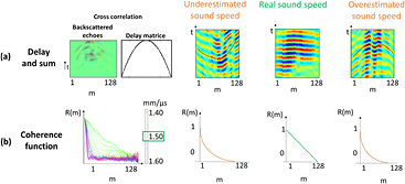
Figure 1. Sound Speed Estimation based on the spatial coherence assessment. An ultrasound pulse is focused at a fixed depth in the medium with an ultrasonic probe. The backscatters echoes are received on the array and their cross-correlations are performed between pairs of transducer elements distant of m elements to compute the coherence function R(m). (a) Flat backscattered echoes, obtained by cross correlation between backscattered echoes and delay matrix, corresponding to different tested speed of sound. (b) Coherence function corresponding to each tested speed of sound. The best speed of sound is the one that provide the highest area under the curve value. When an ultrasound pulse is focused at a fixed depth on the medium, the focal spot is optimized when the precise sound speed is used for the focusing. In this case the coherent function is triangle shape (green curve). When the speed of sound used for focusing is under- or overestimated (orange curve), then the focal spot will increase, leading to a dramatic decrease of coherence.
Download figure:
Standard image High-resolution image2.4.2. Virtual point-like source generation and iterative focusing algorithm for phase aberration correction.
The attainment of an optimal coherence function is possible in a perfectly homogeneous medium with a constant speed of sound. However, sound speed heterogeneities in the intercostal space of difficult patients result in phase aberrations along the travel path of the ultrasonic beam and hinder the precision and robustness of the method. The aim of the second step of our method is to create a virtual point-like reflector in the homogeneous random medium (under the superficial layers) in order to assess the aberrations induced by the medium and improve the precision of our SSE. Indeed, intercostal layers act as near field phase aberrator. In our study, these aberrations are estimated by creating a virtual bright reflector from a random distribution of scattered below the aberrating layer using the concept of iterative time reversal focusing in speckle noise (Montaldo et al 2011) (figure 2) applied on the same RF data used for the previous step. Twenty-five focus beams are virtually emitted in post-treatment at different locations nearby the desired focus (60 mm depth) by recombination of the RF issued from the Hadamard encoded acquisitions (figure 2(a)). In this study, virtual backscattered signals are recorded (figure 2(b)) and 'steered' using the time delays as if all signals were coming from the same reference location (figure 2(c)). The summed corrected backscattered echoes lead to pulsed signals well compressed in time resulting from the created virtual point-like reflector (figure 2(d)). The interested reader should also note that this aberration correction based on time reversal focusing could be performed directly in blood vessels when available following (Osmanski et al 2012).
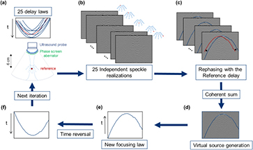
Figure 2. Virtual source generation and iterative focusing algorithm for phase aberration correction. (a) Focused waves are virtually emitted in post-treatment with different delay laws to focus on 25 spots separate by one wavelength. The central point of this grid is considered as the reference point. (b) The echoes (independent speckle realizations) are recorded. (c) Correction of the additional delay compared to the reference central delay. (d) Coherent sum of the speckle realizations after correction of the additional delay, a virtual point reflector emerges. (e) A distorted waveform is obtained. (f) This waveform is time-reversed and injected as the new emission signal in the first step (a) to begin a new iteration.
Download figure:
Standard image High-resolution imageThrough an aberrating layer an iterative algorithm is necessary to converge to a well-defined wave front. In this case, we are going to take benefit on both the isoplanatic patch (Chassat 1989) and the randomness of the scattering medium. When applying the process described earlier to create a point-like reflector in a homogeneous medium, the emitted signals from this virtual bright reflector are no more matching to the heterogeneous medium. So the initial focusing beams are not perfectly focused at their desired locations, however it provides an acceptable start as a first iteration. The new iteration step start replacing the virtually emitted signal from the transducer by the time-reversed version of the signal emitted by the virtual point-like reflector obtain from the first iteration (figure 2(f)). At each iteration the emitted beam profile is improved. After 10 iterations the signal converge to a well-defined wave front. The spatial coherence in random media for the 10th iteration was studied for improving the precision of our SSE.
2.4.3. Superficial layers influence correction.
In addition to the phase aberration correction (heterogeneous local aberrations), superficial layers thickness and speed of sound in these different layers (global averaged aberrations) have to be integrated in the calculation. In this paper, one way of including fat/muscle layers influence correction is studied and discussed: superficial layers thickness measurement.
Thicknesses of fat and muscle layers were measured by the physician with conventional ultrasound. The mean sound speed used in the calculation are 1.450 mm · µs−1 in fat and 1.575 mm · µs−1 in muscle (Azhari 2010). In a multi-layer medium, sound speeds of the different layers are linked by the formula:

Where dtot is 60 mm, ccum the global SSE calculate by the algorithm, dfat the fat layer thickness, cfat the sound speed in fat, dmuscle the muscle layer thickness, dliver = dtot − (dfat + dmuscle), cliver the speed of sound in liver that we aim to determine. cliver is calculated with the formula:

In phantom experiments, superficial layers were mimicked by layers of water with controlled temperature. The CIRS phantom was used (model 054, speed of sound: 1.54 mm · µs−1). Three different water temperatures (cwater) were tested: 37 degrees (cwater = 1.52 mm · µs−1), 20 degrees (cwater = 1.48 mm · µs−1), 14 degrees (c cwater = 1.46 mm · µs−1) (Boed 1999) with different thicknesses from 0 to 26 mm.
2.5. Statistical analysis
A boxplot test was used to study the linear correlation between SSE and biopsy. The mean and standard deviation of the speed of sound were calculated for each Brunt steatosis stage (Grade 0: ⩽10%, Grade 1: 10%–33%, Grade 2: 33%–66%, Grade 3: ⩾66%) (Brunt 2010).
By conventional criteria, a two-tailed p-value under 0.05 was considered to be statistically significant.
Receiver operating characteristic (ROC) analysis was performed in order to evaluate the ability of SSE to be a biomarker for estimating the degree of steatosis. The area under the ROC curve was estimated using the trapezoidal rule. Confidence intervals were stated at a 95% confidence level.
A linear regression was used to study the correlation between SSE and MRI PDFF and R2 is the coefficient of determination and indicates the proportion of the variance in the dependent variable that is predictable from the independent variable.
3. Results
3.1. Sound speed estimation in homogeneous phantoms
A range of sound speed from 1.400 mm · µs−1 to 1.600 mm · µs−1 with a 0.001 step was tested for the ATS phantom (model 551) (figure 3(a)) and for the CIRS phantom (model 054) (figure 3(b)).
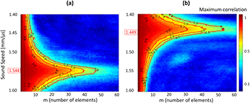
Figure 3. Correlation maps and sound speed estimation (SSE) in two phantoms. Different sound speeds were tested for a 60 mm depth. The correlation maps were calculated in function of the lag in number of elements (m) and the red ISO-value curves are curves of constant minimum value of the maximum correlation for each sound speed (each maximum correlation under one curve is at least equal to the name of the curve). The sound speed characterizing the medium is assuring the highest lag for each minimum of the maximum correlation. (a) SSE was found to be 1.544 mm · µs−1 for the CIRS phantom (model 054). (b) SSE was found to be 1.449 mm · µs−1 for the ATS phantom (model 551).
Download figure:
Standard image High-resolution imageFor each sound speed tested, the maximum correlation was calculated as a function of the lag (in elements). The coherent sum of this maximum correlation was then calculated using equation (2) for each tested sound speed. The SSE value corresponding to the phantom was calculated as the maximum of the polynomial fit of the coherent sum of the maximum correlation. ISO-value curves are another way to visualize the influence of sound speed on the signal coherence. We plotted curves of constant minimum value of the maximum correlation for each sound speed and noticed that the sound speed characterizing the medium is assuring the highest lag for each minimum of the maximum correlation (figures 3 and 4).
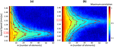
Figure 4. Correlation maps and sound speed estimation (SSE) in two patients. Different sound speeds were tested for a 60 mm depth. The correlation maps were calculated in function of the lag in number of elements (m) and the red ISO-value curves are curves of constant minimum value of the maximum correlation for each sound speed. The sound speed characterizing the medium is assuring the highest lag for each minimum of the maximum correlation. (a) SSE was found to be 1.582 mm · µs−1 for one healthy patient (biopsy 0%, PDFF 2%). (b) SSE was found to be 1.519 mm · µs−1 for one patient with severe steatosis (biopsy 30%, PDFF 8.5%).
Download figure:
Standard image High-resolution imageIn order to find the mean SSE and deviation from the mean for both phantoms and to compare these results with the speed of sound indicated by the constructor, 20 acquisitions with probe repositioning were performed on each phantom. The mean SSE for the ATS phantom was found to be 1.449 ± 0.006 mm · µs−1 for a sound speed given by the constructor of 1.450 mm · µs−1. The mean SSE for the CIRS phantom was found to be 1.544 ± 0.003mm · µs−1 for a sound speed given by the constructor of 1.540 mm · µs−1.
These results demonstrated that in the homogeneous phantom case, the obtained SSE was in good agreement with the speed of sound indicated by the constructor.
3.2. First sound speed estimation in patients
A total of 17 patients with a mean age of 61 years of age (with the total sample set ranging from 30 to 80 years of age), including 30% female and 70% male were examined.
The mean BMI was 26.4 kg · m−2 (range, 21.7–30.5 kg · m−2). One of the 17 patients was obese and 47% (8 of 17) were overweight. No correlation between BMI and MRI PDFF was found (R2 = 0.09) and the technique calculated SSE for all the BMI range. Patients had a mean of 13 mm of subcutaneous fat (range, 4–25 mm). No correlation was observed between thickness of subcutaneous fat layer and MRI PDFF (R2 = 0.16) and the technique calculated SSE for all the thickness range.
For each patient a sound speed range from 1.45 mm · µs−1 (sound speed in pure fat) to 1.65 mm · µs−1 was tested. SSE were calculated the same way as in the phantoms experiments. Correlation maps of two patients with different calculated SSE are presented in figure 4.
We obtained SSE ranging from 1.492 mm · µs−1 to 1.604 mm · µs−1 for patients with MRI PDFF from 2% to 17%, and biopsy from 0% to 80% respectively.
3.3. Sound speed estimation improvement
Studying the coherence function for different sound speed give a global SSE. The aim of this section is now to calculate a local speed of sound in the liver based on the previous SSE. There are two ways of SSE improvement: by correcting the phase aberration induced by the fat and muscle superficial layers, and by taking into account the thickness of these layers.
3.3.1. Phase aberration correction.
Fat and muscle superficial layers act as near field phase screen aberrator. The technique used in this section is based on the aberration correction algorithm. The aim is to straighten the wave front coming from the virtual point like reflector to improve the quality of the focusing. In the case of a patient with a thick superficial fat layer, the phase aberration algorithm succeeds in straightening the wave front and improving the focusing (figure 5).
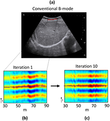
Figure 5. Iterative algorithm for aberration correction. (a) Conventional B-mode of the right sub-costal liver of the patient. A 1 cm thickness fat layer is visible on the top of the liver capsule (hypoechogenic superficial layer). The red line is the superficial aberrating layer shape. (b) Flat backscattered echoes coming for the virtual point like reflector at the first iteration (standard deviation to straight line STD = 0.76). (c) Flat backscattered echoes coming from the same virtual point after 10 iterations of the phase aberration corrective algorithm (standard deviation to straight line STD = 0.26).
Download figure:
Standard image High-resolution imageThe aberration correction algorithm succeeds in improving the focusing quality in every case and in some cases it improves the SSE (figure 6). From iteration 1 to iteration 10, for all patients in this study, a range from 0 to 12% increase in the area under the coherent function curve was measured. For patients with thin superficial layers and mostly composed by muscle, the aberration correction algorithm improves the coherence of the backscattered echoes and confirms the SSE (figure 6, Patient 1). For patients with thick superficial layers and mostly composed by fat, the aberration correction algorithm also improves the coherence of the backscattered echoes but modifies the SSE (figure 6, Patient 2). In both cases, this demonstrate that the first SSE calculated with the VCZ theorem is a robust value leading to the algorithm convergence. This convergence is illustrated by the increase of the area under the VCZ curve (figure 6(c)).
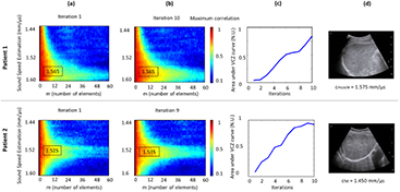
Figure 6. Impact of the aberration correction on the SSE. Results are presented for two patients. (a) Correlation maps at the first iteration. (b) Correlation maps after 10 iterations of the correction aberration algorithm. (c) Evolution of the area under the coherence function curve throughout iterations. (d) Conventional B-mode of the right sub-costal liver. Hypoechogenic superficial layer highlight fat and hyperechogenic superficial layer highlight muscle.
Download figure:
Standard image High-resolution image3.3.2. Superficial layers influence correction.
In this section, one way of including superficial layer thickness into the sound speed calculation is detailed: by superficial layers thicknesses measurement and with a good knowledge of the sound speed in these layers.
To validate the multilayers model in the phantom experiment, we use the thickness of the superficial layer (water at different temperatures) and the sound speed in this layer to correct the SSE. Without layer correction, SSE varies depending on the sound speed in the superficial layer and the thickness of this layer (figure 7(a)). After layer correction the sound speed estimation corresponds to the sound speed given by the constructor (1.54 mm · µs−1) without any dependence with the superficial layer characteristic (figure 7(b)).
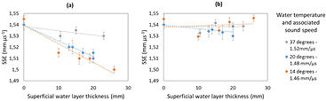
Figure 7. Layer measurement for SSE correction. Error bars for SSE range from ±0.003 to ±0.006 mm · µs−1 and came from a mean over five successive measurements with probe repositioning. (a) Without layer correction, SSE vary depending on the sound speed of the superficial layer and the thickness of this layer. (b) With layer correction, SSE is corresponding to the sound speed given by the constructor (1.54 mm · µs−1).
Download figure:
Standard image High-resolution image3.4. Pilot clinical study results
The aim of this section was to challenge the different steps of SSE calculation and to assess its robustness with two different gold standards, biopsy and MRI PDFF.
Ultrasound and MRI were undergone the same day and MRI and biopsy were undergone with a median of 6 months in between. The first SSE given by the VCZ theorem already gives a proportional relation between MRI PDFF and SSE (R2 = 0.595) (figure 8(a)). As our hypothesis was to find a correlation between the sound speed in the liver (SSE) and the percentage of fat in the latter, we used the coefficient of determination R2 as a relative comparison tool between the different improvement steps. We noticed that aberration correction and superficial layer thickness inclusion in the calculation both improve the proportional relation between MRI PDFF and SSE (respectively figures 8(b) and (c)). With the aberration correction step, aberrations are better taken into account, leading to a higher spatiotemporal coherence of backscattered signals (see figure 6). Consequently, when adding the superficial layers correction, we reached the highest agreement we can obtain so far between MRI PDFF and SEE for this patient cohort (R2 = 0.691) (figure 8(d)).
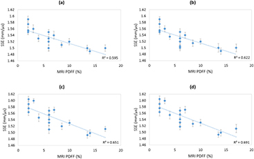
Figure 8. Strong correlation between SSE decrease and MRI PDFF increase. Error bars for SSE range from ±0.007 to ±0.013 mm · µs−1 and came from a mean over four successive measurements with probe repositioning. (a) Step 1: SSE from VCZ theorem. (b) Step 2: SSE including phase aberration correction. (c) Step 3: SSE including superficial layers influence correction. (d) Step 4: optimized SSE including phase aberration correction and superficial layers influence correction.
Download figure:
Standard image High-resolution imageWith the MRI PDFF technique, the cut-off value between healthy and diseased patients was 5% PDFF (Idilman et al 2013) (corresponding to the 10% used in biopsy). SSE was able to significantly differentiate healthy and diseased patients (p < 0.0001, AUROC = 0.942) with an associated criterion of 1.541 mm · µs−1.
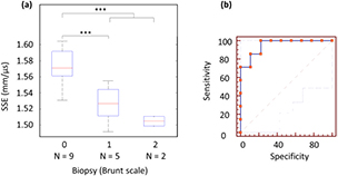
These results are confirmed by the comparison between biopsy and SSE (figure 9(a)). This pilot study demonstrates the SSE ability to significantly differentiate healthy and diseased patients (p < 0.0001, AUROC = 0.952, figure 9) with an associated criterion of 1.555mm · µs−1.
Figure 9. SSE and biopsy comparison with boxplot and ROC curve analysis. (a) Patients are classified in 3 groups according to the Brunt scale. Grade 0 patients are healthy and grade 1 and 2 patients have steatosis. N is the number of patient in each category. The line through the middle of the box represents the median (50th percentile). The top and bottom of the boxes are 75th and 25th percentiles. Significant p value (p < 0.0001) are designated by a star (*). (b) ROC curve analysis to differentiate healthy liver and steatosis with SSE (AUROC = 0.952 (0.719–1.00) 95% CI, p < 104, sensitivity 100% (59.0–100.0) 95% CI, specificity 77.8% (40.0–97.2) 95% CI).
Download figure:
Standard image High-resolution image
4. Discussion
In this study, we introduced a method for precise and robust in vivo sound speed assessment. The technique was firstly validated on two phantoms. In the case of homogeneous phantom the SSE found was in good agreement with the speed of sound indicated by the constructor (Phantom 1, cconstrucor = 1.450 mm · µs−1 and SSE = 1.449 ± 0.006 mm · µs−1; Phantom 2, cconstrucor =1.540 mm · µs−1 and SSE = 1.544 ± 0.003 mm · µs−1).
Secondly, in the pilot clinical study, the potential of this method for noninvasive liver steatosis detection and staging was proved. Our approach enables an accurate estimate of the ultrasonic sound speed in the liver with a standard deviation below 5%. We obtained SSE ranging from 1.492 mm · µs−1 to 1.604 mm · µs−1 for patients with MRI PDFF from 2% to 17%, and biopsy from 0% to 80% respectively. MRI PDFF and biopsy were used as gold standards with a particular attention to MRI PDFF, as it is to date considered as the most efficient approach for steatosis estimation (Idilman et al 2013). It is even considered better than liver biopsy as this latter is hindered by the non-negligible possibility to miss a steatosic region leading to false negative values (Sumida et al 2014). Moreover, as demonstrated by Leporq and colleagues (Leporq et al 2014), by giving access to the percentage of fat protons regarding to the percentage of water protons, MRI PDFF allow a linear steatosis staging, instead a groups classification like biopsy.
Our method is based on a three steps processing in order to guarantee accuracy. The first step provides an estimate of the sound speed optimizing the spatial coherence of backscaterred speckle noise. As this estimation can be degraded by aberrations occurring during propagation in the first layers, a virtual point like reflector is created in order to find and correct these aberrations. This aberration correction technique was found to be efficient as it allows in many cases (N = 14) to increase the AUC of the spatial coherence function of the region of interest (a ratio increase of AUCiteration1/AUCiteration10 = 6% ± 1%). Finally a third correction step is introduced in order to correct the bias introduced by the intercostal layer thickness for an optimal estimation of liver sound speed. This third step, tested on multilayer phantom experiments improve SSE robustness by including superficial layers thickness in the calculation.
These successive steps lead to a very high linear correlation (R2 = 0.691) between MRI PDFF and SSE and therefore enable to grade hepatic steatosis. Moreover, SSE was excellent to significantly differentiate healthy and diseased patients (p < 0.0001, AUROC = 0.942).
As a second confirmation, ROC curve analysis was performed to test the ability of SSE to differentiate healthy liver and steatosis with biopsy as gold standard (p < 0.0001, AUROC = 0.952). This analysis leads to the conclusion that SSE is able to diagnose healthy liver and steatosis as well as biopsy. Our technique can establish cutoff value between healthy patients and patients with steatosis (SSEcriterion = 1.555 mm · µs−1).
SSE strength is its ability to grade steatosis like MRI PDFF. Moreover, with both MRI PDFF and biopsy as gold standards, SSE was demonstrated to be valuable for hepatic steatosis 10% or greater detection, which is critical in patient who undergo living donor liver transplantation because of the risks of poor graft survival, initial graft dysfunction, and other complications (Trotter et al 2007, Sharma et al 2013).
Our ultrasound based method has the advantage to provide a more easy-to-use and accessible imaging modality for the screening of liver steatosis. Moreover, it could be combined with stiffness (Young's Modulus) measurements using Shear Wave Elastography (Deffieux et al 2015) or radiation force Shear Wave Speed estimation (Palmeri et al 2005).
Some authors see the interference caused by thoracic subcutaneous fat as the limiting factor for success in obese patients (Foucher et al 2006a). However as we included the thickness of the superficial layers and the phase aberration correction, our technique was found to be robust for all patients of this preliminary proof of concept study.
A limitation of this study is the population heterogeneity. Some patients had chronic liver diseases with various degree of fibrosis or even cirrhosis. As a preliminary study the role of fibrosis was not studied as a confounding factor, but another study with a larger patient cohort is planned to study fibrosis as a confounding factor for sound speed estimation by ultrasound.
5. Conclusion
This study proposes a robust method for sound speed estimation (SSE) in homogeneous and heterogeneous medium. This technique was first validated on two phantoms. The use of sound speed as a hepatic steatosis biomarker was then proposed and demonstrated in a preliminary clinical evaluation. In vivo sound speed was assessed using an ultrasound-based method combining speckle noise coherence analysis and an aberration correction technique. It was found to be highly correlated with MRI Proton Density Fat Fraction and biopsy results. This non-invasive technique was implemented on a research ultrasound scanner and could be combined with Shear Wave Elastography for global fibrosis and steatosis grading.
Acknowledgment
The authors kindly thank J Robin for proofreading the manuscript grammar. This work was supported by the Agence Nationale de la Recherche under the program 'Future Investments' with the reference ANR-10-EQPX-15 and by LABEX WIFI (Laboratory of Excellence ANR-10-LABX-24) and the French Program 'Investments for the Future' under reference ANR-10-IDEX-0001-02 PSL*. This work was also partly supported by the European Research Council under the European Union's Seventh Framework Programme (FP7/2007–2013)/ERC Advanced grant agreement 339244 FUSIMAGINE).