

Abstract
The well-being of the ever-escalating world population hinges largely upon the adequacy of clean, fresh water. Desalination is one of the most promising approaches in such an endeavor. Using molecular dynamics simulations, we take a close look at nanoporous hexagonal boron nitride nanosheets as desalination membranes, and study how C dopants affect their performance. The calculations predict that the desalination performance of C-doped BN membranes compares favorably to that of MoS2 membranes: the water flux through the 0% (0CB–0CN), 25% (3CB–0CN), 75% (3CB–6CN), and 100% C terminated BN membrane (6CB–6CN) is 29.9, 47.5, 95.3, and 81.5 molecules ns−1 per pore, respectively, and there is a strong correlation between the water flux and the axial diffusion coefficient. Through our study of the effect of C content on the desalination performance, it is found that more clustering of water molecules at membrane pores due to a smaller hydration free energy and pore energy barrier assists water transport through the pores, and allows a greater water flux.
Export citation and abstract BibTeX RIS
1. Introduction
The escalation of population and rise of industrialization in numerous regions of the world, especially developing countries, place inundating strain on the supply of fresh water [1–4]. Indeed this has severely endangered the livelihood and survival of mankind—approximately 1.2 billion or 15% of the world's population still does not have access to drinking water [5], and yet, water demand is predicted to climb at twice the rate of population growth [6]. The number of people affected has been forecast to rise to 3.9 billion in the coming decades [7].
Desalination of seawater is one of the most promising approaches to alleviate the problem of water shortage since seawater is abundant in supply (97.5% of all water on earth), and the desalination process does not upset the ecological and hydrologic systems. Although desalination has provided 38 billion cubic meters of water in year 2016—a twofold increase over that in 2008, it is still insufficient for our needs. As austere as it sounds, the scarcity of portable water has aggravated to a point such that traditional clean water technologies including those used in desalination are no longer adequately efficacious to meet the demands, and the high capital costs of old infrastructure call for an urgent revamp of its design.
In most desalination plants, clean water is produced by applying pressure to force solvent molecules across a semi-permeable membrane in a process known as reverse osmosis (RO). The applied pressure has to be sufficiently large to overcome the osmotic pressure of the solvent. The membrane also blocks the transport of salts or other solutes. In contrast, forward osmosis (FO) (or simply osmosis) is the spontaneous movement of solvent molecules from a solvent to another with a higher osmotic pressure [2, 8, 9]. Despite the need to apply an external pressure in RO, its total energy consumption is usually lower than in FO due to the absence of an evaporation step. However, FO has a few advantages over RO, including lower and reversible membrane fouling [2, 10, 11], higher salt rejection [12, 13], and less contamination in the feed solution [2, 14–19].
The osmotic membrane acts as the most important 'cog' in the desalination 'machinery'; solvent- and solute-membrane interactions dictate the permeability of these molecules through the membrane in the osmosis process. Novel designs of membrane seek to enhance the energy efficiency of desalination [20, 21], and at the same time attain a greater water flux and salt rejection. Advances in nanotechnology allow membranes to be synthesized from materials such as carbon nanotubes (CNTs) [22], and nanoporous monolayers, including graphene [23], graphene oxide [24], molybdenum disulfide (MoS2) [25], and boron nitride (BN) [26]. These thin low-dimensional materials are pliant in form, facilitating integration with other components of the desalination plant. Nevertheless, the desalination performance is divergent among many of these materials; although they have a similar composition, CNTs exhibit lower salt rejection than graphene [27]. On the other hand, water can permeate at a similar rate in materials of a different composition, albeit of the same atomic arrangement, for instance in BN nanotubes and CNTs [28]. Despite the greater adaptability of monolayer materials in plant design, multilayer materials are often more economical to synthesize. More configurational variables also exist for multilayer membranes than for monolayer ones, such as layer separation and nanopore offset [29], which then allow larger margins of adjustment in optimizing the performance trade-off between the osmotic flux and ion rejection. To this end, multilayer materials might fare better in desalination membranes.
Essential in these mono- and multi-layer membranes, nanopores constitute the sieve channels through which solvent molecules pass osmotically between the draw and feed chambers. The geometrical construct and chemical composition of the pores govern the interaction strength between the pore atoms and solvent/solute molecules, and consequently, the permeability of these molecules. In this case, the selectivity of the osmotic membrane can be facilely and effectively manipulated by precise decoration of the pores. Recent advances in lithography techniques facilitate the fabrication of nanoporous membranes [30, 31], however the precision of site-specific doping remains as the main experimental challenge. Although BN nanotubes fare reasonably well in desalination with respect to CNTs [28], BN multilayers realize a smaller water flux than graphene multilayers due to a larger friction force and energy barrier at the pores [32]. BN multilayers notwithstanding, have other strengths over their carbon counterparts, such as higher oxidation resistance [33]. Therefore, the question lies in whether we can have 'the best of both worlds'. In this computational study, we add C dopants to the pores of nanoporous hexagonal boron nitride membranes, and peruse their effects on the desalination performance, including the significance of doping site on the water transport. An external pressure difference and an osmotic pressure difference between the two chambers of saline solution drives the solvent and ion transport through the membrane by RO. In contrast to most modeling studies [29, 34], we investigate the RO performance when the initial permeate solution is saline instead of being freshwater, and at a lower salinity than the initial feed solution. The water transport is characterized by its flux through the membrane pores, and its axial diffusion coefficient. Two approaches are employed to calculate free energies: (1) exponential averaging in the single-topology paradigm to obtain the effective hydration free energy of each membrane, and the hydration free energy of each element type in the pores; and (2) thermodynamic integration to steer a water molecule towards each pore type to derive the potential of mean force (PMF) profile along the pulling path, and thereby the free energy barrier at the pore. In the latter approach, we first vary the pulling speed to systematically search for an appropriate force constant for subsequent steered calculations. The degree of hydration of each species is also described by the number of water molecules in their first hydration shell as determined from the pair distribution functions. The oxygen density profiles charting the trajectories of the water molecules entering and exiting through the pores further delineate the interaction between the water molecules and the pores.
2. Computational details
2.1. Geometrical structure
The membrane was placed between a reservoir of a saline solution (feed solution) with (30 Na+/30 Cl−: 57.3 g l−1) ions and 1600 water molecules, and another reservoir of a saline solution (permeate solution) with (21 Na+/21 Cl−: 40.8 g l−1) ions and the same number of water molecules. The salinity of both solutions was relatively higher than that of seawater (35.0 g l−1), and they are considered as brine solutions. It is not uncommon that solutions used in simulation studies have higher NaCl concentrations than in desalination plants to ensure sufficient interactions of salt ions with the membrane, given a limited simulation time [35]. The initial 'water box' was created by VMD [36] and TopoTools [37]. Two pristine hexagonal BN (hBN) monolayers were introduced as piston walls to apply a hydraulic transmembrane pressure on the solutions—every piston atom on the side of the solution with a greater osmotic pressure was given a larger force towards the membrane than each atom of the other piston. An external pressure of 500 MPa was applied, which is commonplace in modeling studies [29]. As described in [29], the water flux is linearly proportional to the applied pressure, and therefore can be extrapolated down to pressures typical in operating conditions (∼5 to 10 MPa) in RO desalination plants. The unit cell of the system measured 2.6 nm × 2.7 nm × 51.0 nm, with the z-dimension perpendicular to the plane of the membrane (figure 1(c)). Four pores (of two different types depending on the terminating atoms, P1 and P2), each 24.65 Å2 in area, were created in the desalination membrane. We chose four different membrane configurations, which varied in the type of terminating atoms—100% pore termination by C (hereby known as 6CB–6CN), 0% C termination (0CB–0CN) (which is essentially nanoporous hBN), and the intermediate structures containing 75% C termination (3CB–6CN) and 25% C termination (3CB–0CN) (figure 1). The membrane configuration is denoted by □CB–□CN, which refers to the number of terminating B and N atoms substituted by C atoms. We define terminating atoms to be those that are not fully coordinated at the pore, and in this case, those that have one less coordinated atom. For example, '25% C Term (3CB–0CN)' refers to a nanoporous membrane with 3 terminating B atoms substituted by C atoms. Considering only 1 P1 pore and 1 P2 pore, there are in total 6 terminating B atoms and 6 terminating N atoms. 3 atomic substitutions out of 12 atoms constitute 25% C termination. These configurations are also specially chosen (1) to vary the C content, and also (2) to compare between substitutional doping of pore B and N atoms. In this case, in increasing degree of doping, from 0CB–0CN to 3CB–0CN, three pore B atoms are replaced by C atoms; from 3CB–0CN to 3CB–6CN, six pore N atoms are substituted by C atoms; from 3CB–6CN to 6CB–6CN, the last three pore B atoms are C-doped.
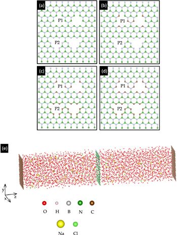
Figure 1. Atomic structure of four different membrane configurations—(a) 0% C termination (0CB–0CN), (b) 25% C termination (3CB–0CN), (c) 75% C termination (3CB–6CN) and (d) 100% C termination (6CB–6CN). B, N, and C atoms are denoted in green, white, and brown, respectively. P1 and P2 label the two types of pore. (e) Snapshot of the (6CB–6CN) system. Atoms in red: O; pink: H; silver: B; green: N; brown: C; yellow: Na; light green: Cl. The feed chamber lies to the left of the membrane, while the permeate chamber lies to the right of it.
Download figure:
Standard image High-resolution image2.2. Molecular dynamics
Due to the size of the system (which includes the membrane, pistons, and water) and the time scale to allow the capture of the event of diffusion, force-field techniques are required. The MD simulations were performed using the large-scale atomic/molecular massively parallel simulator [38]. The four-site transferable intermolecular potential with 4 points (TIP4P) was used for water molecules [39], and the SHAKE algorithm constrained and reset the bond lengths and angles after each timestep. The covalent bonds between B, C, and N atoms are modeled by the Tersoff potential [40]. The interactions between water, salt ions, and the membrane included van der Waals and electrostatic terms. The van der Waals interaction was represented by the 12-6 Lennard-Jones potential ![$4\varepsilon [{(\sigma /r)}^{12}-{(\sigma /r)}^{6}]\,.$](https://content.cld.iop.org/journals/0957-4484/30/5/055401/revision2/nanoaaf063ieqn1.gif) Some parameters were given in [41–43], and others derived from the Lorentz–Berthelot combining rules [44] [εB–O = 0.005 27 eV, σB–O = 3.322 Å; εN–O = 0.00650 eV, σN–O = 3.278 Å; εC–O = 0.00491 eV, σC–O = 3.275 Å].
Some parameters were given in [41–43], and others derived from the Lorentz–Berthelot combining rules [44] [εB–O = 0.005 27 eV, σB–O = 3.322 Å; εN–O = 0.00650 eV, σN–O = 3.278 Å; εC–O = 0.00491 eV, σC–O = 3.275 Å].
The atomic charges on the atoms and ions were:  = −1.0484,
  = −0.5242,
  = 1.0000,
  = −1.0000,
  = 1.0500,
  = −1.0500. In the work by Won et al [41], the charges of ±1.05e for B and N respectively may have overestimated the electrostatic interaction, and hence the water flux may be realistically larger than what has been calculated in this paper. On the other hand, C atoms are modeled as uncharged particles, similar to what has been implemented in [32]. The Lennard-Jones potential was truncated at 1.3 nm and the long-range Coulomb interactions are computed using the particle–particle particle-mesh (PPPM) algorithm [45]. The timestep of equation of motion was 0.5 fs. The Nosé–Hoover thermostat [46] was used to control the temperature. Periodic boundary conditions were applied in all directions, which were mandatory for the implementation of the PPPM algorithm. The length of the simulation cell in the direction perpendicular to the membrane was chosen to be slightly greater than twice that of the initial water box to ensure that there was no periodic continuity from the opposite wall of the cell during osmotic flow of the particles through the membrane. As the hBN piston walls were non-porous, the chamber of water and salt ions were sealed up along its axis. These piston walls moved freely and equilibrated to adjust to the pressure exerted on them.
2.3. Free-energy calculations: exponential averaging
The thermodynamics of water transport across desalination membranes are characterized by the hydration free energy and the energy barrier at the membrane. One of the earliest formalisms of free energy calculations is derived from the perturbation theory. In the free energy perturbation (FEP) [47], or more accurately the exponential averaging method, there are two systems, one of which is the unperturbed or the reference one, and the other is the perturbed or the target one. The Hamiltonian of the perturbed system is represented as the sum of the reference Hamiltonian and a perturbation term. An order parameter is a collective variable that describes transformations from the initial reference system to the final target one, and can be either a function of atomic coordinates or a parameter in the Hamiltonian. The former type of order parameter corresponds to the transformation path and marks the progress of a reaction by Newtonian equations of motion, hence it is named the reaction coordinate or the reaction path. Alas, the task of defining the reaction coordinate analytically is often non-trivial. In such a case, the order parameter is then approximated by simpler analogs. Parameterization via the Hamiltonian is no less tricky as such a parameter does not naturally propagate via Newtonian dynamics.
In FEP, the free energy difference between an  -particle reference system with a Hamiltonian
  (
( is the Cartesian coordinate, and
  is the corresponding momenta) and a target system described by
  is denoted by
  The difference in the Helmholtz free energy
  can be written as a ratio of the corresponding partition functions, and conventionally, it is expressed as a cumulant expansion with respect to the probability distribution of finding the reference system in a particular state,

where  is the
  th cumulant of
2.4. Free-energy calculations: steered molecular dynamics (SMD)
Another approach to determine the free energy behavior of water transport is SMD [48, 49], which applies external steering forces or constraints (e.g. harmonic potentials) in certain degrees of freedom to steer molecules along a prescribed path in the configuration space. This accelerates processes that are usually too slow due to energy barriers, and therefore allows us to explore these processes on time scales which are accessible to molecular dynamics simulations. The PMF is the free energy profile along the reaction coordinate, and is determined through the Boltzmann-weighted average over all degrees of freedom except the reaction coordinate. In the constrained scenario of SMD, the PMF describes the diffusive motion of the molecule along the reaction coordinate. However, SMD is a non-equilibrium process, while PMF is an equilibrium property. Jarzynski's equality mediates between the two, allowing the calculation of free energies from non-equilibrium processes. It relates the external work  done on a system during a transformation between two equilibrium states and the Helmholtz free energy difference
  between the two states:

where  and
and  is the Boltzmann constant. In actual molecular dynamics simulations, the accumulated work done is usually employed to approximate the exponential averaging.
3. Hydration number
The pair distribution function  or radial distribution function, describes the time-averaged influence of an atom on the disposition of neighboring atoms. In other words, it describes the probability of finding atoms of a particular species at a distance r away from a reference atom, i.e. the density as a function of distance from the reference atom. The cumulative integral of
 gives the coordination number of the species from the reference one. Figure 2 shows the
  and
and  of B, N, and C atoms with respect to the O atoms of the water molecules, in each of the four membrane configurations. Distinction is made between the membrane atoms terminated at the pores and at non-porous regions; to illustrate, the configuration in figure 1(a) contains 18 atoms terminated at the pores. Moreover, figure 2 shows the
  and
and  of C atoms substituting either B or N atoms at the pores. The value of the function
  at the first minimum of
  denotes the hydration number, or the number of water molecules that can solvate an ion, of that species within its 1st hydration shell. Note that consideration is given to statistical errors in the derivation of
  which affects the exact position of the 1st minima. In this case, a slight trough in
  is ignored, and only a significant dip is accepted as the minimum.
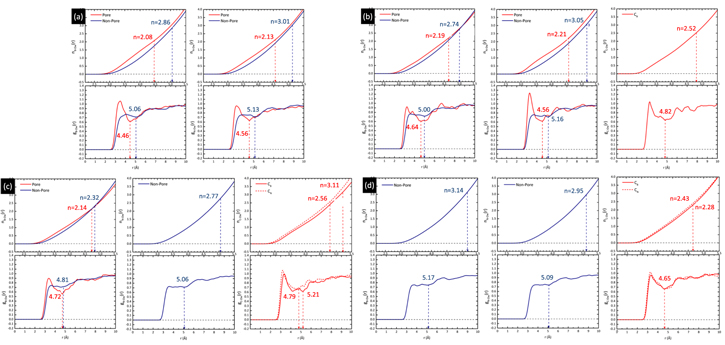
Figure 2. B/N/C–O Pair distribution functions  and their cumulative integral
  of four different membrane configurations—(a) 0% C termination (0CB–0CN), (b) 25% C termination (3CB–0CN), (c) 75% C termination (3CB–6CN) and (d) 100% C termination (6CB–6CN). The vertical dashed lines mark the demarcation between the 1st and 2nd hydration shell. Distinction is made between the membrane atoms terminated at the pores and at non-porous regions; for example, the configuration in figure 1(a) contains 18 atoms terminated at the pores.
Download figure:
Standard image High-resolution imageThe 1st minima for all the different species are located relatively far from the reference atom at above 4 Å. Regardless of the presence of C dopants, terminating B and N atoms at the pores have smaller 1st hydration shells, and lower hydration numbers than atoms at non-porous regions, for instance, hydration number of 2.08 (pores) against 2.86 (non-porous) in the undoped membrane (0CB–0CN). This suggests that it is less favorable energetically for water molecules to be located near pores than at non-porous regions. It is also observed from figure 2 that doping the pore with C atoms increases the hydration number within the 1st hydration shell. As the hydration number is often inversely related to the free energy required to hydrate any atom, we shall readdress this in section 6 regarding the effect of doping on the hydration free energies. For now, we note that naively, if we were to take the average of the 1st hydration number for each membrane, considering only 1 pore P1 and 1 pore P2 (12 pore atoms in total), the 75% C terminated membrane has the largest 1st hydration number, i.e. there is most clustering of water molecules, followed by the 100%, 25%, and then 0% C terminated membranes. Moreover, the slow climb of  to unity and its flatter, lower, and less distinct leading peak at the non-porous regions imply a loose packing of the water molecules within its 1st hydration shell, and a non-distinct segregation between the hydration shells. This is especially apparent in comparison to the
  at the pores. The calculations for the average 1st hydration number follow:


4. Trajectory of water molecules through pores
Figure 2 describes the atomic coordination of water molecules at the pores and non-porous regions.  and
and  are statistically derived over a period of time by radial packing of atoms around any reference one—the orientation of atomic pairs is disregarded. Therefore, these metrics lack dynamical information of water transport through the porous membranes. On the other hand, an oxygen density profile depicts an n-dimensional view of the probability of locating an oxygen atom. Akin to the previous section, the oxygen atoms are representative of the water molecules [50–52]. 3 slabs of equal thickness (1.0 Å) near each pore are designated to sample the oxygen density: (1) the topmost color maps in figure 3 are drawn from the slabs in the feed chamber, and in front of the pores (i.e. before diffusion through the membrane); (2) the bottommost maps are obtained from the slabs in the permeate chamber; and (3) the maps in the middle are calculated from the slabs sandwiched between those in the feed and permeate chambers. In other words, the center slabs encompass the pores, and span across the two water chambers. Taking z-axis as the longitudinal axis along which diffusion occurs, (1) ranges from z = −1.5 to −0.5 Å, (2) ranges from z = 0.5–1.5 Å, and (3) ranges from z = −0.5 to 0.5 Å.
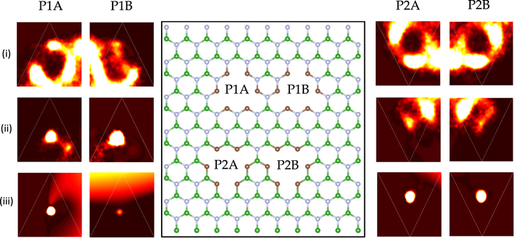
Figure 3. Oxygen density profile (i) in the feed chamber of 100% C terminated (6CB–6CN) membrane near the pore, (ii) at the pore, and (iii) in the permeate chamber near the pore. A lighter shade corresponds to a higher density.
Download figure:
Standard image High-resolution imageThe probable positions in the slabs as derived from the oxygen density profiles plot the favorable trajectories of water molecules as they leave the feed chamber and enter the permeate chamber. The oxygen density profiles are highly similar in the four membrane configurations, suggesting that the trajectories of the water molecules are not contingent on the atomic content of the pores. In a representative case of the fully C-terminated 6CB–6CN membrane (figure 3), water molecules either (1) prefer to leave the feed chamber nearer two of the three edges of the triangular pores, or (2) are bound more strongly to these two edges in the static sense. These two edges are positioned closer to the neighboring pores than the remaining edge; in any of the two above scenarios, atoms in neighboring pores have a strong influence on water molecules in the feed chamber. In realistic settings, water molecules are less likely to deviate from the axis through the center of the pores due to two reasons: (1) the symmetrical geometry of each pore with respect to neighboring ones in large membranes with more pores (I.e. a desalination membrane has many more pores than what has been simulated. In that regard, most pores have neighboring pores around them, and therefore the effect of neighboring pores on the oxygen density would be diminished.), and (2) the larger spacing between pores. Nevertheless, the simulations in this study show that the exit path of the water molecules from the feed chamber is not affected by the type of atoms the pore contains.
Water molecules tend to diffuse through the center of the pores (figure 3), or between the two edges that are close to the neighboring pores. Unlike the strong attraction from atoms in neighboring pores before they pass through the pores (figure 3(i)), they are concentrated along the axis through the pore centers upon entering the permeate chamber, albeit slight differences between the corresponding pairs of pores (i.e., P1A-P1B, P2A-P2B, figure 3(iii)). Similar phenomena observed in all four membrane configurations (refer to supporting information, which is available online at stacks.iop.org/NANO/30/055401/mmedia) according to their oxygen density profiles attests to the insignificance of the type of terminating atoms on the trajectory of water molecules in the desalination chambers. However, it is yet unclear to us why neighboring pores only affect the exit paths from the feed chamber and not the entrance paths into the permeate chamber.
5. Water transport: flux and axial diffusion coefficient
The performance of desalination membranes is typically characterized by the diffusivity of water molecules across the membrane and the ability of the membrane to reject ions. An efficient membrane allows fast diffusion of water molecules from the feed chamber into the permeate chamber, and forbids ions, usually Na+ and Cl−, from passing through the membrane. In our simulations, the number of water molecules and salt ions in each chamber is tracked for a total of 15 ns. It has been found that the simulation time of 15 ns is sufficient for all 1600 water molecules in the feed chamber to diffuse into the permeate chamber for each membrane configuration.
The net number of water molecules (per pore) that has crossed the membrane for the entire duration of 15 ns is presented in figure 4(a). The linearity of each plot before it levels off is indicative of a constant water flux during desalination, and is testament to the stability of the RO process. Averaging the net number of filtered molecules across time, the water flux through the 0% (0CB–0CN), 25% (3CB–0CN), 75% (3CB–6CN), and 100% C terminated membrane (6CB–6CN) is 29.9, 47.5, 95.3, and 81.5 molecules ns−1 per pore, respectively. We compare these values with those reported for nanoporous MoS2 membranes with an external pressure of 250 MPa (this study: 500 MPa); it ranges from 120 to 165 molecules ns−1 per pore, depending on the type of pore termination (Mo, S, or mixed), albeit at more than twice the pore size of between 55.45 and 57.38 Å2 (this study: 24.65 Å2) [34]. Fitting the water flux to the size of Mo-only pores at 250 MPa in [34] yields the equation  approximately, where
  is the water flux in molecules ns−1, and
  is the pore area. This gives a water flux of 36 molecules ns−1 per 24.65 Å2 Mo-only pore at 250 MPa. This is approximately 70 molecules ns−1 when scaled to 500 MPa, and therefore, C-doped BN membranes perform well relative to MoS2 membranes. We do not compute the permeability coefficient, since the model for these coefficients assumes linearity between the external pressure and the water flux, which is found to be true only at small external pressures as reported in [34].
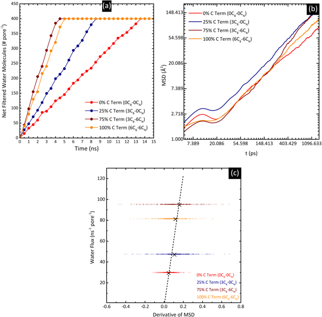
Figure 4. (a) Net filtered water molecules, (b) mean square displacement, and (c) correlation between water flux and the derivative of mean square displacement of four different membrane configurations—0% C termination (0CB–0CN), 25% C termination (3CB–0CN), 75% C termination (3CB–6CN) and 100% C termination (6CB–6CN). The dashed line in (c) shows the linearity of the correlation. The linearity of (a) before it levels off shows that the water flux during desalination is constant. An initial bump appears in (b) at approximately 10 ps, before increasing steadily.
Download figure:
Standard image High-resolution imageWater molecules permeate the membrane by diffusion, hence the diffusion rate along the direction of desalination directly relates to the water flux across the membrane. The axial diffusion coefficient can be calculated from the derivative of the mean square displacement (MSD) of the water molecules, which in turn measures the deviation of the position of the atoms with respect to their initial position over time

where  is the axial diffusion coefficient,
  is the dimensional factor (
 = 2, 4 and 6 for 1D, 2D and 3D diffusion, respectively),
  is the time, and
  denotes the atom coordinates. The MSD with respect to time in natural logarithm (ln) scale shows an initial bump at approximately 10 ps, before increasing steadily (figure 4(b)). The bump likely originates from the fluctuation of the particles when they are equilibrating. Recording in the ln scale reveals details not easily perceptible in the linear scale. Since the derivative of MSD gives the diffusion coefficient, a membrane allowing a constant water flux should ideally have a constant derivative of MSD. Indeed, figure 4(c) shows that the water flux of each membrane (figure 4(a)) correlates linearly with the mean value of MSD derivative (i.e. diffusion coefficient) obtained from figure 4(b).
At the end of the 15 ns simulation for every membrane configuration, the number of salt ions in each chamber remains unchanged, i.e. the salt rejection ratio is 100%. Small MoS2 pores of similar sizes (approximately 18 Å2) have also recorded perfect salt rejection efficiencies [34]. Unlike the flux of water molecules, the rejection of salt ions depends more on the pore size than on the pore content [34]. Therefore, the pore size of 24.65 Å2 used in this paper is deemed suitable to explore the desalination potential of C-doped BN membranes. We recommend that in the pursuit of optimizing the water flux in desalination membranes, pores are made to sizes similar to the aforementioned to avoid compromising the ability to reject ions.
6. Hydration free energy
Alchemical transformations computationally alter one chemical species into another, essentially allowing us to realize the age-old dream of matter transmutation. FEP is one of the most common approaches for these transformations, and has been employed in various physical chemistry and biochemistry problems, including solvation properties [53], protein-ligand binding [54], protein folding [55], and conformational equilibria [56].
The sequence of alchemical transformations is designed to restore the system to its initial state in a thermodynamic cycle, hence the total change of free energy is zero. Since the system is in thermodynamic equilibrium at every point in the cycle, the transformations are reversible, i.e. both forward and backward routes reap the same results. However, it is usually computationally more efficient to compute a particular free energy in one of the two directions, and there are small errors between free energies along the two FEP paths. Figure 5(a) shows the thermodynamic cycle of the hydration of pores. There are two routes to calculate the hydration free energy of pores  —the first is via the systems 1 → 2 → 3, and the second is via 1 → 4 → 5 → 6 → 3, as denoted in figure 5(a). System 1 only contains the membrane and salt ions. Water molecules are then added in system 2. As our interest is in the hydration free energy of the pores, and not the salt ions, the interactions between the water molecules and the salt ions are decoupled in system 3. System 4 describes the annihilation of the pore atoms from system 1, whilst system 5 adds water molecules, which interact with the salt ions. Finally, system 6 removes the interaction between the water molecules and the salt ions. Using 1 → 4 → 5 → 6 → 3, the hydration free energy can be calculated by either of the two paths
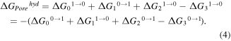
Figure 5. (a) Thermodynamic cycle of the hydration of pores, (b) mean of the free energy differences taken along the forward and backward paths of the thermodynamic cycle, and (c) contribution of each pore atom type to the hydration free energy. The first of the two routes in (a) to calculate the hydration free energy of pores is via the systems 1 → 2 → 3, and the second is via 1 → 4 → 5 → 6 → 3. The order parameter λ in (b) is varied between 0 and 1.
Download figure:
Standard image High-resolution imageFigure 5(b) compares the free energy differences of the pores in each membrane configuration taken along the thermodynamic cycle (figure 5(a)) as the order parameter λ is varied between 0 and 1. The energies are means of the forward and backward paths in the thermodynamic cycle. The alchemical transformations are carried out in the single-topology paradigm; atoms are annihilated (created) by progressive reduction (increase) of their van der Waals parameters. The discrepancy between the free energies in both paths is less than 9%, which is considered trivial and insignificant. The value of the order parameter 0 and 1 refers to the state of systems 1 and 3 in figure 5(a), respectively. The free energy difference at λ = 0 has been adjusted to zero to facilitate comparison (figure 5(b)). In other words, we assume that the free energy difference of each membrane configuration is identical in the absence of water molecules (system 1, figure 5(a)). The hydration free energy is negative for all membranes, suggesting that water stabilizes every membrane. The energy is −0.130, −0.111, −0.082, and −0.105 eV for the 0CB–0CN, 3CB–0CN, 3CB–6CN, 6CB–6CN membranes, respectively. The least amount of energy is required for the pore in the 3CB–6CN membrane to hydrate, which results in clustering of most water molecules at the pores (figure 2), and hence facilitates the transport of water molecules through the pores. This indirectly explains its largest water flux recorded among the four membrane configurations.
The contribution of each pore atom type (per atom) to  is tabulated in figure 5(c). N atoms generally have larger
  than B atoms, e.g. in the 0CB–0CN membrane. On the other hand, C atoms substituting N sites have significantly greater hydration free energies than C atoms substituting B sites, e.g in the 6CB–6CN membrane. For instance, CB atoms in the 3CB–6CN membrane has a free energy of −2.379 meV while that of CN atoms is almost 80% larger (in absolute terms) at −4.362 meV. It is apparent pore N atoms are hindering the hydration of the pores—complete doping of N atoms by C atoms in the 3CB–6CN membrane marks a relative 34% drop in
  from the 3CB–0CN membrane; in contrast, there is only a slight decrease in
  of the B and CB atoms. However, as more C atoms are added to dope B atoms in the 6CB–6CN membrane,
  of the C atoms (CB and CN) increases considerably to raise the effective hydration free energy of the membrane.
Apparently, the C content is not the definitive factor governing how well the membrane hydrates; the site of doping, which relates to its chemical environment, plays a critical role too. Unlike the hydration number (section 3), the hydration free energy does not increase monotonously with the amount of C dopants. Figure 5(b) predicts that a combination of B atoms and C dopants (e.g. 3CB–6CN in our selection of configurations) at the pore favors the minimization of the effective hydration free energy. We believe that membrane configurations such as 2CB–6CN and 4CB–6CN will record similar values of hydration free energy.
7. Free energy barrier at pores
Two SMD simulations are carried out for each membrane configuration and pore type. A single water molecule is positioned in the feed chamber with its O atom 5 Å away from the pore center, and along the pore axis. The PMF of the system is tracked as the water molecule is pulled towards the pore center. As it travels along its trajectory, the steered water molecule quickly orientates itself among other water molecules to minimize interaction forces. Therefore, the initial position of its H atoms with respect to its O atom is trivial, and it is given the same orientation in each SMD simulation. Constrained molecular dynamics, one method of which is SMD, is chosen instead of simply deriving the PMF from the logarithm of  because it yields free energies of higher accuracy than the latter; in the latter, a relatively small change in the free energy corresponds to large changes in
  thereby often incurring substantial inaccuracies.
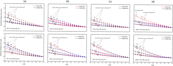
What would then be an appropriate spring constant for the driving force? This is decided by making several trial runs at different spring constants (in this study 0.5, 1.0, 2.0 kcal mol−1 Å−2), and identifying the upper bound below which a change in the pulling speed (0.001, 0.0005 Å fs−1) does not vary the PMF profile. Figure 6 collates the PMF profile of each membrane configuration and pore type. There is only a slight discrepancy between the profiles of different pulling speed at the spring constant of 0.5 kcal mol−1 Å−2, implying that this spring constant is suitable in these steering simulations. For a fair comparison between the various simulations, and since a slower pull is considered more accurate to capture the dynamics in thermodynamic integration, the PMF profiles at a pulling speed of 0.0005 Å fs−1 are considered in this study.
Figure 6. Potential of mean force profiles at spring constants of (A) 0.5, (B) 1.0, (C) 2.0 kcal mol−1 Å−2, and pulling speeds of 0.001 (in red), 0.0005 Å fs−1 (in blue) towards Pores 1 (P1, top) and 2 (P2, bottom) of membranes of (a) 0% C termination (0CB–0CN), (b) 25% C termination (3CB–0CN), (c) 75% C termination (3CB–6CN) and (d) 100% C termination (6CB–6CN). Several trial runs were made at the aforementioned spring constants to identify the upper bound below which a change in the pulling speed does not vary the PMF profile.
Download figure:
Standard image High-resolution image
The PMF value calculated at the center of the pore denotes the energy barrier the water molecule needs to overcome as it is pulled along its path towards its destination. Figure 6 shows that a stiffer spring (larger spring constant) poses a larger energy barrier at the pores. At the spring constant of 0.5 kcal mol−1 Å−2, and taking the average of the two pore cases, the PMF experienced at the pore center is 0.55, 0.45, 0.33 and 0.37 eV, for the 0CB–0CN, 3CB–0CN, 3CB–6CN, and 6CB–6CN membranes, respectively. The trend of these values is consistent with that of the predicted water flux, hydration free energy, hydration number, and also diffusion coefficient.
8. Conclusion
Industrialization is a double-edged sword—most developing nations witness a rapid hike in their quality of living, but they also face the dire need to find more clean, fresh water to sustain their growing population. In this molecular dynamics study, we investigate the effects of C dopants on the desalination performance of nanoporous hexagonal boron nitride membranes, including the significance of doping site on the water transport. Our calculations show that doping atoms at the pores with C atoms increases their hydration number. The trajectory of water molecules does not depend on the atomic content of the pores. The desalination performance of C-doped BN membranes is predicted to be comparable to that of MoS2 membranes. The water flux through the 0% (0CB–0CN), 25% (3CB–0CN), 75% (3CB–6CN), and 100% C terminated membrane (6CB–6CN) is 29.9, 47.5, 95.3, and 81.5 molecules ns−1 per pore, respectively, at 500 MPa, and it correlates well with their axial diffusion coefficient. Moreover, it is found that a membrane allowing a greater water flux has a smaller hydration free energy and energy barrier at the pore, and has more clustering of water molecules at the pore (i.e. greater hydration number), thereby suggesting that clustering of water molecules at pores assists water transport through the pores. It is also evident that the slower water flux of the 100% C terminated membrane as compared to the 75% one arises due to the additional energy barrier introduced by the 6 additional CB atoms. The calculations have verified that the salt rejection ratio of each membrane configuration remains at 100% at the pore size of 24.65 Å2.
Acknowledgments
The author gratefully thanks the A*STAR Computational Resource Center (ACRC) for the computing time.