
Abstract
Metals deform plastically at the asperity level when brought in contact with a counter body even when the nominal contact pressure is small. Modeling the plasticity of solids with rough surfaces is challenging due to the multi-scale nature of surface roughness and the length-scale dependence of plasticity. While discrete-dislocation plasticity (DDP) simulations capture size-dependent plasticity by keeping track of the motion of individual dislocations, only simple two-dimensional surface geometries have so far been studied with DDP. The main computational bottleneck in contact problems modeled by DDP is the calculation of the dislocation image fields. We address this issue by combining two-dimensional DDP with Green's function molecular dynamics. The resulting method allows for an efficient boundary-value-method based treatment of elasticity in the presence of dislocations. We demonstrate that our method captures plasticity quantitatively from single to many dislocations and that it scales more favorably with system size than conventional methods. We also derive the relevant Green's functions for elastic slabs of finite width allowing arbitrary boundary conditions on top and bottom surface to be simulated.
Export citation and abstract BibTeX RIS

Original content from this work may be used under the terms of the Creative Commons Attribution 3.0 licence. Any further distribution of this work must maintain attribution to the author(s) and the title of the work, journal citation and DOI.
1. Introduction
Modeling the contact mechanics of solid bodies assuming realistic surface roughness is highly relevant to tribology, the science of friction. This is a demanding task, because the height spectra of most surfaces, even polished ones, have non-negligible magnitude over several decades of wavelengths, typically from the atomic scale to several dozen or even hundreds of microns [3, 4], i.e., the root mean square heights are determined by the longest-wavelength height fluctuations (relevant for sealing and lubricant flow) while the root mean square gradients (relevant for typical contact stresses, at least in the elastic limit) are determined by the shortest wavelengths. In the past years, various theories of rough surface contact have been presented [5–10]. Persson's contact-mechanics theory [8–10] appears particularly promising to us, because it accounts for long-range elastic deformations, unlike traditional approaches such as those inspired by Greenwood and Williamson [6], who pursued local bearing models. In fact, Persson theory reproduces quite well experiments and numerical results on relative contact area, interfacial stress distribution functions, stress spectra, and gap distribution functions, although it requires a fitting parameter of order unity. However, the validity of Persson's analysis of plastic contacts [9] in the range where plasticity is size-dependent [11–14] has not yet been shown.
Numerical simulations of contact between elastic rough surfaces are made possible through several techniques. Of particular interest are the boundary-element based approaches such as BEM [15–17] and Green's function molecular dynamics (GFMD) [18–22], which calculate the response of a solid to contact loading by modeling only the surface. These methods are suitable to study large systems where the surface roughness is described by many orders of length scale [2, 20, 23]. In this work, we choose GFMD over BEM, since it is a simpler method, which does not involve solving the Fredholm integral equations. In GFMD, the equilibrium positions of the interfacial grid points are found by means of damped dynamics in Fourier space, where the individual modes decouple. This allows for large systems to be quickly brought to equilibrium. While the computational complexity of BEM scales with  , where n is the number of discretization nodes, GFMD scales as
  . Furthermore, it is straightforwad in GFMD to employ non-holonomic boundary conditions and/or interaction potentials between the contacting bodies and hence it is cost-effective in studying problems where the contact area is not known a priori. Conventional FEM or BEM methods typically require several iterations as well as incremental updating of the boundary conditions in order to converge to a final contact area. Additionally, GFMD has the advantage that it can be extended to a multi-scale method [24] where the surface layer can be described atomistically and the substrate underneath be treated within the harmonic approximation. Pastewka et al [24, 25] have shown that the elastic Green's function can be quickly computed from interatomic potentials and a seamless coupling to the atomic region can be derived even for interactions going beyond nearest-neighbor interactions. GFMD has been successfully used to model the contact response of semi-infinite elastic solids [2, 26, 27], while plasticity was neglected.
There has also been much progress in the numerical study of elasto-plastic contacts. These, however, are either based on continuum plasticity [28–30], or, limited to single-wavelength roughness [31], or, based on brute-force all-atom approaches [32, 33]. To date, no studies of rough surface contact appear to have disseminated, in which (size-dependent) plasticity and long-range elasticity were both accurately modeled. Our work aims at building such a model.
Size-dependent plasticity in metal crystals has been successfully predicted by discrete dislocation plasticity (DDP) [1] simulations, which for simple problems, as the tensile response of free-standing metal films, give results in quantitative agreement with experiments [34]. In the context of contact mechanics, DDP has been used to study indentation of flat surfaced single crystals with single indenters [35, 36], periodic indenters [37, 38], as well as an indenter with self-affine surface modeled as a collection of Hertzian contacts [39]. The only DDP studies, in which the plastically deforming bodies were not approximated to be flat, involved the flattening of simple sinusoidal surfaces [40–42]. Results showed that the contact area is not continuous, but serrated, as a consequence of dislocations exiting the surface through discrete slip planes and leaving crystallographic steps. Due to the serrated nature of the contact area, the local contact pressure presented high spikes, at odds with the pressure profiles predicted by continuum plasticity. The study of size-dependent plasticity for realistic surface geometries is computationally very expensive. In order to being able to study indentation using realistic surface geometries, we here combine the accurate description of plasticity offered by DDP with the fastly converging elastic solution delivered by GFMD, in a modeling technique which we name Green's function dislocation dynamics (GFDD). This is not the first attempt to combine dislocation dynamics with a boundary element method [43–46]. However, for realistic surface geometries coming into contact, which require a fine discretization, GFDD should be more cost-effective. This is because the method relies on fast Fourier transform (FFT) and employs damped dynamics to quickly equilibrate large systems.
We begin the paper by briefly introducing DDP in section 2 and GFMD in section 3. We then present the methodology of the new model in section 4. The results obtained using the new GFDD model are compared with DDP in sections 5 and 6. Section 7 summarizes the advantages and potentials of the new method.
2. Discrete dislocation plasticity
DDP is a numerical technique to solve boundary-value problems (b.v.p), which treats plasticity as the collective motion of discrete dislocations [1]. The dislocations are modeled as line defects in an elastic continuum. The solution at each time step of the simulation is obtained by the superposition of two linear elastic solutions: the elastic fields for dislocations in a homogeneous infinite solid, and the solution to the complementary elastic b.v.p., which corrects for the boundary conditions. The methodology is illustrated for the indentation of a single crystal by an array of flat rigid indenters in figure 1. The elastic dislocation fields are represented by a superscript ( ), the fields solving the complementary b.v.p. by a superscript
  . The elastic dislocation fields are given analytically. The dislocation in the repetitive cell and its periodic replicas are treated as an infinite array of dislocations. The solution to the b.v.p. is traditionally obtained using the finite-element method FEM. The rigid indenter is modeled implicitly by imposing boundary conditions on the deformable body.
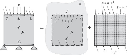
Figure 1. Schematic representation of the DDP methodology: the boundary-value problem for a body containing dislocations is decomposed into two parts: the fields of the dislocations in an infinite medium and the solution to the elastic boundary-value problem which corrects for the boundary conditions.
Download figure:
Standard image High-resolution imageThe total stress and displacement fields obtained at a given time increment are used, along with a set of constitutive rules, to describe the evolution of the dislocation structure. The constitutive rules are based on the Peach–Koehler force and control dislocation glide, nucleation, annihilation and pinning at obstacles. At the beginning of the simulation, the crystal is dislocation-free, but contains a density of point sources and obstacles that mimic Frank–Read sources and precipitates, respectively. The density of sources and obstacles is constant during the simulation. A dislocation pair is generated by a point source when the resolved shear stress acting on the source exceeds a critical nucleation strength,  . The dislocation then glides on a plane with a velocity proportional to the Peach–Koehler force. Two dislocations with opposite Burgers vector annihilate when they come closer to each other than a threshold length, set to
  , where b is the magnitude of the Burgers vector. Whenever a dislocation meets an obstacle it gets pinned. It is released by the obstacle only when the Peach–Koehler force acting on the dislocation exceeds the critical strength of the obstacle,
  . Dislocations can exit the domain through the free surface leaving behind a displacement step of
  along the slip direction.
The aim of this work is to replace the FEM solution to the complementary b.v.p. with GFMD, while the constitutive rules that control the dislocation dynamics remain unchanged and similar to those proposed in [1].
3. Green's function molecular dynamics
GFMD is also a boundary-value method to study the elastic response of a body subjected to contact loading. In GFMD, only the surface of the deformable body is modeled explicitly and discretized using equi-spaced grid points as seen in figure 2. The grid points, under the influence of an external load, are displaced from their initial position, causing an increase in the areal elastic energy of the system. The new equilibrium positions are then calculated using damped dynamics in Fourier space. The advantage of damping the system in Fourier space is that the different modes describing the surface are uncoupled, and the stress–displacement relationship, when applying a load in z-direction, simply reads:

where  is the Green's function tensor,
  is the α component of the displacement and and
  is the traction in β-direction corresponding to wavenumber
  . The Green's function tensor depends on the elastic properties and size of the body.
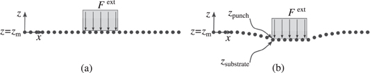
Figure 2. Schematic representation of a rigid punch indenting a flat deformable body: (a) the undeformed configuration and (b) the deformed configuration.
Download figure:
Standard image High-resolution imageHere, the load is applied in an incremental manner by means of a rigid flat indenter, which is modeled by a hard-wall potential. To satisfy static equilibrium at each incremental change of the loading, the following condition must hold:

where  is the external force;
  is the interfacial force ensuring the non-overlap constraint, which are imposed 'by hand' after each time step, in real space,
  is the elastic restoring force that can be written as:

where A0 is the total surface area and  is the inverse Green's function, which can be evaluated from the areal elastic energy density
  . The areal elastic energy was derived for a slab with deformable top and fixed bottom in previous works [47, 48]. In section 4.1, we extend the derivation to the case where the bottom surface can be exposed to arbitrary stress, displacement, or mixed boundary condition. This is necessary for the coupling to dislocation dynamics, as should become clear in the following section.
The damping force has the form:

where η is the damping factor, chosen such to critically damp the slowest mode, i.e., the center-of-mass mode, corresponding to q = 0, for quick convergence. Various further improvements can be applied to speed up convergence, such as, mode-dependent masses or damping.
The damping force is used in the position-Verlet algorithm to solve for the displacement fields at each increment  ,
,

where τ is the non-dimensional discrete time step used in the simulation.
The hard-wall potential is employed at the end of each iteration to ensure there is no inter-penetration, i.e., in real space,

where  and
and  are the z-coordinates of the punch and substrate surface, respectively as seen in the figure 2. Notice that the method is not bound to use a hard-wall potential. Finite interactions can be accounted for, however, we have here chosen for a hard-wall potential for the sake of comparison to conventional DDP.
When the surface equilibrates to the final deformed configuration, the body fields are calculated from the discrete surface fields using closed-form analytical solutions [48].
4. Green's function dislocation dynamics
The GFDD method is based on the same decomposition concept as used in DDP except that, now, the image fields are found using GFMD instead of FEM. The methodology is schematically presented in figure 3 for the case of a layer indented using a flat rigid punch. Note that GFDD can solve generic boundary value problems where both top and bottom boundaries are arbitrarily partitioned into traction and displacement boundaries.
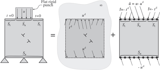
Figure 3. Decomposition of the problem for the dislocated body similar to figure 1 except for the complementary problem, which is solved using GFMD.
Download figure:
Standard image High-resolution imageWhen solving the complementary b.v.p., both tractions and displacements caused by the dislocations on the top and bottom boundary of the body need to be simultaneously prescribed at a given time increment. Tractions are imposed in Fourier space as described in the previous section by using  as external force
  before stepping forward in time. Here
  is the Fourier transformation of the discontinuous function
  at point
  :
:

where St and Su are traction- and displacement-prescribed boundaries, respectively. Unlike tractions, displacements are imposed in real space by setting the equilibrium position of the hard-wall to the required position:

The hard-wall is not applied to the boundaries where traction is prescribed  .
.
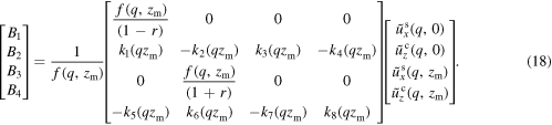
Notice that the elastic energy required for the evaluation of the Green's function, which is needed in the calculation of the restoring elastic force, was derived in [48] but only for the case of an isotropic slab with an undulated top layer and a fixed bottom. This allows a b.v.p. to be solved for a mixed boundary condition at the top, however, with the restriction of the bottom displacement to be zero. Here, however, we need to impose mixed boundary conditions also at the bottom. To this end, the areal elastic energy is required for a solid with both top and bottom undulation as seen in figure 4. This will be dealt with in the subsequent section.
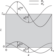
Figure 4. Periodic unit cell of an isotropic slab of height  represented by the shaded region is undulated at the top and bottom surfaces in lateral and normal directions.
Download figure:
Standard image High-resolution image4.1. Elastic energy of an elastic layer loaded at both surfaces
A linear elastic isotropic body in a slab geometry is considered. The equilibrium condition for the case of no body forces can be written as  , where
  is the stress at point (x, z) represented by vector
  and
and  . This can be written as:
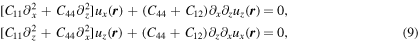
where  denotes the coefficients of the elastic tensor. The in-plane wavenumber q is a scalar for the two-dimensional body considered here.
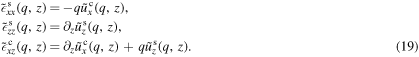
It is shown in appendix A that for the system of differential equations (9) the solutions of the in-plane cosine transform of the lateral ux displacement field couples to the in-plane sine transform of the normal uz displacement and vice versa. Thus, we can write:

Solutions satisfying the following boundary conditions:
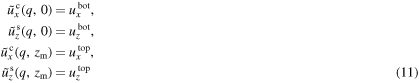
and equation (9) are then obtained to satisfy
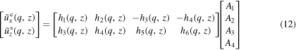
with
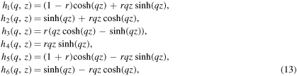
where  and
and  . Ai can be found by applying the boundary conditions in equation (11):
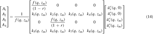
with
and
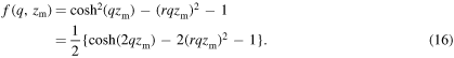
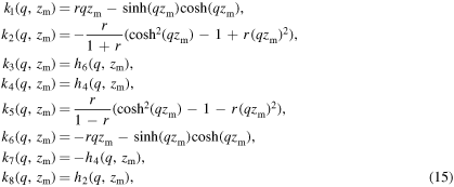
Similarly, the in-plane sine transform of ux and cosine transform of uz can be obtained from:
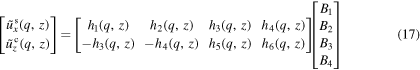
with
From equation (12), the strains are calculated as:
Stresses are then obtained as usual through Hooke's law:

Gathering all contributions to the elastic energy leads to
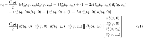
with
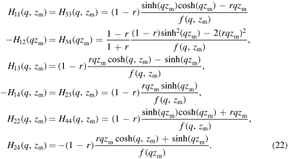
The complete elastic energy density containing the complex Fourier transform of the displacement with wavenumber q reads
with
The body fields are obtained through the closed-form analytical expressions in equations (12) and (17). The displacement fields hence obtained are compared with those obtained by FEM in figures 5 and 6. The relative difference in the displacement field obtained using both methods are found to be below 0.25%. It has to be noted that periodic boundary conditions in GFMD are intrinsically enforced through the periodicity of the Fourier transforms. In FEM, periodicity can be imposed using various methods, including the penalty method, as done in this study, or Lagrangian multipliers, but is never exact.
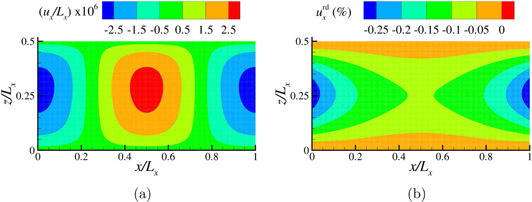
Figure 5. Lateral displacement ux in an elastic layer with undulations  ,
,  ,
,  and
and  obtained using (a) GFMD and (b) the relative difference map with
  .
.
Download figure:
Standard image High-resolution image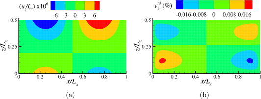
Figure 6. Normal displacement uz in an elastic layer with undulations  ,
,  ,
,  and
and  obtained using (a) GFMD and (b) the relative difference map with
  .
.
Download figure:
Standard image High-resolution imageThe elastic energy density in equation (23) is extended to the case of a semi-infinite half-space in appendix B. This opens up the possibility of modeling the plastic contact response of a semi-infinite body using dislocation-dynamics simulations. This is beneficial to study the plastic response of a body under contact loading without the effect of its bottom, i.e., an increase in contact pressure caused by dislocations piling up at the bottom of the body.
5. Preliminary results: a simple static solution
In this section, the new GFDD model is compared to DDP when computing the image fields for the simplest case scenario: a single dislocation pinned in an isotropic slab with Young's modulus E = 70 GPa and Poissons ratio  . The magnitude of the Burger's vector is
  .
.
Simulations are carried out for a unit cell with the bottom fixed and a traction free top surface, i.e.,

The stress distribution obtained using GFDD is compared with DDP in figure 7. The displacements at the top surface, where tractions are zero, and the tractions at the bottom surface, where displacement are zero, are shown in figures 8 and 9.
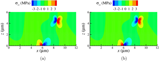
Figure 7. Stress fields for a dislocated elastic layer with a traction free top surface obtained using (a) GFDD and (b) DDP.
Download figure:
Standard image High-resolution image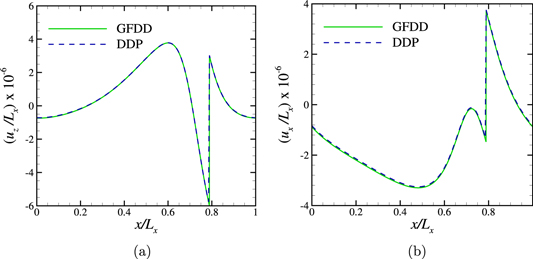
Figure 8. (a) Normal displacement uz and (b) lateral displacement ux at the traction free surface of an elastic layer containing a pinned edge dislocation obtained using GFDD and DDP.
Download figure:
Standard image High-resolution image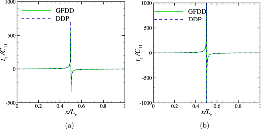
Figure 9. (a) Lateral traction tx and (b) normal traction tz at the bottom surface of the elastic layer containing a pinned edge dislocation obtained using GFDD and DDP.
Download figure:
Standard image High-resolution imageIt is found that the tractions at the surface obtained using GFDD suffer from ringing, also known as Gibb's phenomenon (see figure 10). This is because the discontinuities in the displacement imposed at the surfaces cause the higher harmonics of the traction to have higher amplitudes than the lower harmonics. To remove the ringing artifacts the results displayed in figure 9 are obtained after multiplying the traction  with a sinc function
  , where a0 is the discretization length. This is equivalent to convolving in real space the traction suffering from ringing with a rectangular box of unit height and width equal to the discretization length. Notice, however, that ringing affects only surface tractions, not surface displacements, from which the body fields are calculated.
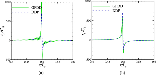
Figure 10. Lateral traction tx at the bottom surface (a) before and (b) after the removal of ringing artifacts.
Download figure:
Standard image High-resolution image6. Indentation by an array of flat rigid punches
This benchmark problem is used to compare GFDD to classical DDP. The simulations are carried out for a unit cell that is indented by a rigid punch as in figure 11.
Figure 11. Boundary-value problem.
Download figure:
Standard image High-resolution image6.1. Boundary-value problem
The indentation is prescribed by specifying the normal displacement rate along the contact of length  :
:
A sticking contact is modeled in DDP by taking the lateral displacement ux = 0 in the contact region. In GFDD, the lateral movement in the contact region is constrained horizontally through the hard-wall potential. The non-contact part of the top surface of the unit cell is taken to be traction-free,

This is achieved in GFDD by letting the contact points relax to equilibrium without any constraints. Finally, the bottom of the unit cell, z = 0 is fixed:
In GFDD, this is implemented by constraining the lateral and normal motion of grid points at the bottom surface using the hard-wall potential.
6.2. Choice of parameters
Calculations are carried out for crystals with aspect ratio  , contact fractions
  and
and  . The elastic constants are chosen to represent aluminum: the Young's modulus is E = 70 GPa and Poissons ratio
  .
.
For the DDP simulations, the slab is discretized using a uniform mesh of square elements. The number of degrees of freedom is  , where nnx is the number of nodes in x-direction, and nnz the number of nodes in z-direction. For the GFDD simulations, the surface is discretized using nx equi-spaced grid points, with nx = nnx.
In GFDD, the center-of-mass mode is critically damped or slightly under-damped for quick convergence. The damping factor η is

where τ is the non-dimensional time step shown earlier in equation (5) that is used in the position-Verlet algorithm in GFMD to solve for the unknown displacement fields and it is taken to be τ = 0.25. The number of iterations used to reach convergence scales as  .
.
The dislocations can glide on three sets of parallel slip planes, with slip plane orientations:  and 120◦ to the top surface. The discrete slip planes are spaced at
  where
where  is the length of the Burger's vector. The Frank–Read sources and obstacles are randomly distributed in the crystal with a density
  and
and  in an initially dislocation free crystal. The strength of the sources follows a Gaussian distribution with mean strength
  and standard deviation of
  . The critical time for nucleation is
  . The strength of the obstacles is taken to be
  . Dislocations of opposite sign in the same slip plane annihilate when the distance between them is below
  . The time step in both DDP and GFDD simulations is taken to be
  ns.
ns.
6.3. A simple dislocation dynamic simulation: a single Frank–Read source
In this section, a simple problem is considered where a rigid flat punch indents a crystal containing a single Frank–Read source as shown in figure 12(a). In order to observe appreciable plastic deformation in the material, the magnitude of the Burger's vector is magnified four times, i.e.,  . The mean contact pressure obtained using both methods is displayed in figure 12(b). While the flat rigid punch indents the layer, the source keeps generating dislocation dipoles, causing periodic kinks in the pressure–displacement curve. The difference in mean contact pressure in figure 12(b) is not seen to the naked eye.
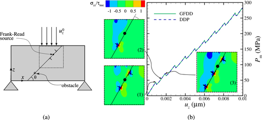
Figure 12. (a) Schematic representation of the problem with a single Frank–Read source lying on a slip plane at an angle θ with the surface of the crystal. (b) Mean contact pressure for  . The dislocation structure and stress distribution is shown at three different depth of indentations: (1) when the first pair of dislocation is nucleated, (2) when the first dislocation exits and (3) when the second dipole is nucleated.
Download figure:
Standard image High-resolution imageThe surface fields obtained using both methods at  are shown in figure 13. The displacement steps formed due to the exiting of dislocations can be clearly seen close to
  .
.
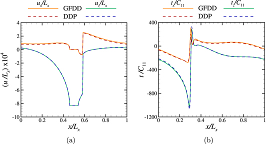
Figure 13. (a) Displacement at the top surface and (b) traction at the bottom surface obtained using GFDD and DDP at the final indentation depth  . The green curve in (a) overlaps with the blue-dashed curve since displacement boundary conditions are prescribed in the z-direction.
Download figure:
Standard image High-resolution imageNote that in figure 13(a) the curves for the uz displacement overlap since in z-direction displacement boundary conditions are imposed. The difference between the curves representing ux stems from the numerical difference in calculating the resolved shear stress acting on the source and the location of the dislocations in the two numerical schemes. The calculated stress field depends not only on boundary conditions when the simulation is elastic, but also on the location of other dislocations in the crystal when there is plasticity. Therefore, the differences builds up with increasing dislocation density. However, relative differences between contact pressure claculated in figure 13(b) with two methods remain below  .
.
6.4. Dislocation dynamics simulation with many sources and obstacles
In this section the indented crystals contain a density of Frank–Read sources  and a density of obstacles
  . The simulations are carried out with DDP and GFDD on crystals containing the same realization of sources and obstacles, i.e., the location as well as the strength of sources and obstacles are identical. Figure 15 shows the stress state and dislocation distribution at final indentation depth. Note that there is no one-to-one correspondence between the dislocations and therefore also not in terms of stress distribution. This is not surprising given that a tiny difference in the evolution of the dislocation structure, like a small delay in the nucleation of a dislocation or in the formation of a junction, would trigger an avalanche of differences in the following dislocation dynamics [49]. The overall features such as the shear bands emitted by the contact are captured by both methods in the same way. This is also testified by the mean contact pressure in figure 14(a) for the simulation presented in figure 15 and for a different realization. While DDP and GFDD do not produce identical mean pressures as a function of displacement for a given realization of Frank–Read sources, differences tend to be larger within one method from one realization to the next. In figure 14(b) are presented the average between the three realizations.
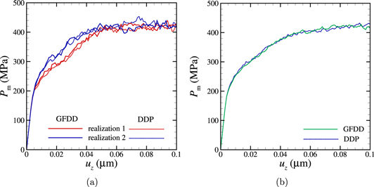
Figure 14. Mean contact pressure  obtained using GFDD and DDP for
  are plotted for (a) two different initial realizations of dislocation structure and (b) average of three different realizations.
Download figure:
Standard image High-resolution image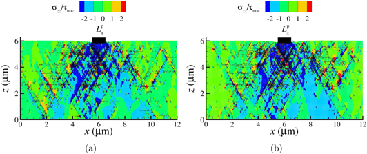
Figure 15. Stress and dislocation distribution in the crystal for the first realization obtained using (a) GFDD and (b) DDP for an indentation depth  and
and  .
.
Download figure:
Standard image High-resolution image6.5. Simulation time
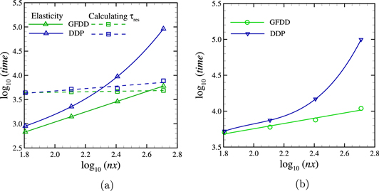
The computational complexity involved in solving the elastic b.v.p. using GFDD is only  [48], while it is
  [50] in DDP, where B is the mean bandwidth of the stiffness matrix, which cannot exceed nx.
The time consuming part in 2D dislocation dynamics is the calculation of the resolved shear stress  at the location of objects, i.e., sources, dislocations and obstacles. In DDP, this requires searching the element where the object is located and subsequently calculating the stress and interpolating it to the location of the object. This procedure scales as
  . In GFDD, instead, the resolved shear stress can be evaluated directly at the points of interest, i.e., at dislocations, sources and obstacles, which requires a smaller computational effort, scaling with O(nx). This is because the body field is calculated based on surface displacements
  using
using  modes.
The simulation time required for elasticity and for the calculation of the resolved shear stress is displayed in figure 16, and shows in both cases how the computational advantage of using GFDD increases with increasing discretization. It has to be noted that we use a skyline solver for FEM. The computational time using this solver was found to be of the same order as that of iterative solvers. The simulations performed on a single Intel Xeon(R) 3.10 GHz processor with 31.3 Gbytes of RAM.
Figure 16. (a) Simulation time (in seconds) for the elastic boundary-value problem and calculating resolved shear stress  are plotted separately, (b) total simulation time including dislocation dynamics for GFDD versus DDP for the full simulation.
Download figure:
Standard image High-resolution image
The dislocation dynamics is computed using the same algorithm in both methods and takes therefore the same amount of time and resources. The time required for the dynamics is independent of the discretization and increases with dislocation density. For the DDP simulations performed here, the time consumed by the dislocation dynamics is a negligible fraction of the time required to compute the resolved shear stress. GFDD is thus computationally more efficient than DDP independently of dislocation density.
It has to be noted that the maximum number of surface nodes chosen for this study is only 29. If one intends to study the contact response of a realistic self-affine surface where roughness scales over three orders of magnitude ranging in scale from 50 nm to 100 μm [3], the surface has to be discretized by at least 213 points (or even more depending on the thermodynamic and continuum limit [2]). For such large systems, and small strain simulations, as typically used in dislocation dynamics, the computational complexity for elastic b.v.p. was found to always dominate in comparison to the dislocation dynamics. In this case the computational advantage of GFDD becomes even more appreciable.
Notice also that the benchmark problem chosen in this work involves a constant contact area. For contact problems where the area is not constant, DDP becomes even slower since finding the correct contact area by means of the FEM requires many iterations as well as updating the boundary conditions at each time increment. GFDD is inherently impervious to such issues since it employs an interaction potential between the contacting surfaces.
7. Concluding remarks
In this work, we propose a modeling technique, GFDD, which combines GFMD with DDP. We firstly extended the existing GFMD model such that it can simulate an elastic layer with arbitrary loading at both the top and bottom surfaces. To this end we derived the areal elastic energy for the case of an isotropic layer with sinusoidal loading at both ends. In addition, we derived the body fields required to capture the evolution of the dislocation structure. The results obtained using GFDD are compared with conventional DDP for a benchmark problem: periodic indentation of a single crystal by flat punches.
The mean contact pressure during indentation using the two methods is found to differ less than two different realizations using the same method. Here by realization is intended a given initial distribution of dislocation sources and obstacles. The differences between the two methods stems from the evaluation of the fields using different discretizations: GFDD discretizes only the surface, DDP also the body.
The new GFDD model has various advantages compared to classical DDP. First, it is faster and opens up the possibility of studying realistic rough surfaces by exploiting a larger number of degrees of freedom. Next, GFDD employs an interaction potential between the contacting bodies, and does not involve time-consuming algorithms to keep track of the evolution of the contact area. Also, the periodicity in GFDD is intrinsically enforced through Fourier transforms, making it a better candidate than DDP to study contact problems by exploiting the periodicity of the unit cell on which the analysis is performed. Obviously, this is also a limitation of the GFDD model, which is currently not suitable to study non-periodic problems. Extension of the model to overcome this limitation seems an interesting avenue for future research. Additionally, the GFDD model has the potential to serve as a platform for multi-scale modeling where the surface has an explicit atomistic description and the bulk can be treated as a dislocated continuum.
Acknowledgments
This project has received funding from the European Research Council (ERC) under the European Union's Horizon 2020 research and innovation programme (grant agreement no. 681813). LN also acknowledges support by the Dutch National Scientific Foundation NWO and Dutch Technology Foundation STW (VIDI grant 12669).
Appendix A.: Lateral-normal displacement coupling
It was shown in [48] that assuming an in-plane undulation of the top surface of an isotropic layer with a real-valued wavenumber q, equation (9) can be solved with the factorization

Substituting equation (A.1) in the equilibrium condition (9), it can be rewritten in Fourier space as

Equation (A.2) then reduces to

This implies that

This explains how the solutions of the in-plane cosine transform of the lateral ux displacement field couples to the in-plane sine transform of the normal uz displacement, and vice versa.
Appendix B.: Asymptotic analysis
For the limiting case in which the height of the slab tends to infinity,  can be written as:
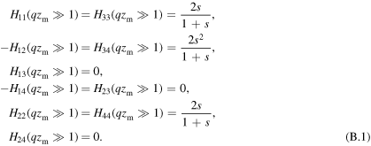
In the limiting case of short wave-numbers, we find
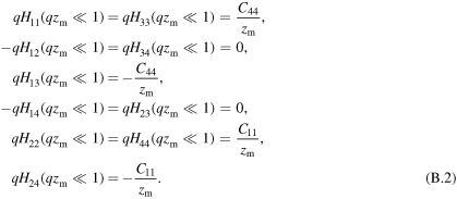
In the case of bottom undulation going to zero  , we recover the elastic energy for a fixed bottom derived in [48].