

Abstract
As measurements of velocity and temperature fields are of paramount importance for analyzing heat transfer problems, the development and characterization of measuring techniques is an ongoing challenge. In this respect, optical measurements have become a powerful tool, as both quantities can be measured noninvasively. For instance, combining particle image velocimetry (PIV) and particle image thermometry (PIT) using thermochromic liquid crystals (TLCs) as tracer particles allows for a simultaneous measurement of velocity and temperature fields with low uncertainty. However, the temperature dependency of the color appearance of TLCs, which is used for the temperature measurements, is affected by several experimental parameters. In particular, the spectrum of the white light source, necessary for the illumination of TLCs, shows a greater influence on the range of color play with temperature of TLCs. Therefore, two different spectral distributions of the white light illumination have been tested. The results clearly indicate that a spectrum with reduced intensities in the blue range and increased intensities in the red range leads to a higher sensitivity for temperature measurements, which decreases the measurement uncertainty. Furthermore, the influence of the angle between illumination and observation of TLCs has been studied in detail. It is shown that the temperature measurement range of TLCs drastically decreases with an increasing angle between illumination and observation. A high sensitivity is obtained for angles in between  and
and  , promising temperature measurements with a very low uncertainty within this range. Finally, a new calibration approach for temperature measurements via the color of TLCs is presented. Based on linear interpolation of the temperature dependent value of hue, uncertainties in the range of 0.1 K are possible, offering the possibility to measure very small temperature differences. The potential of the developed approach is shown at the example of simultaneous measurements of velocity and temperature fields in Rayleigh–Bénard convection.
Export citation and abstract BibTeX RIS

Original content from this work may be used under the terms of the Creative Commons Attribution 3.0 licence. Any further distribution of this work must maintain attribution to the author(s) and the title of the work, journal citation and DOI.
1. Introduction
With regard to challenges caused by the change of climate, analysis of heat transfer in the atmosphere and oceans become more and more important [1, 2]. This heat transfer is significantly determined by natural convection, induced by temperature differences leading to a varying density of a fluid. Therefore, numerous investigations covering simulations [3, 4] and experiments [5] were performed on a reduced scale, to characterize the evolving mechanism in natural convection. For this, the velocity and temperature field in Rayleigh–Bénard systems, as a simplified model on a reduced scale, were analyzed [6, 7]. Furthermore, velocity and temperature fields are also of great interest for many technical aspects, as for example the design of heat exchangers [8]. In order to understand the correlation of those fields in detail, simultaneous measurements are necessary. With regard to the velocity measurements, the particle image velocimetry (PIV) has established as state of the art, because this technique offers a noninvasive measurement of velocity fields with high temporal and spatial resolution [9, 10]. In order to measure temperature fields simultaneously, several techniques have proved to be successful, depending on the application. For example, combining laser induced fluorescence (LIF) with PIV is a suitable approach to measure velocity and temperature fields at the same time [11, 12]. For this, a temperature sensitive dye is dissolved in the fluid additionally, while tracer particles are suspended in the fluid for velocity measurements according to the principle of PIV. However, the particles interfere with the temperature measurements, causing a higher uncertainty for the scalar quantity [12]. While LIF is based on fluorescent dyes, there are other measuring techniques that use the same tracer particles for the determination of the velocity and temperature field. One approach is the use of thermographic phosphor tracer particles doped with rare-earth ions, that act as luminescent activator centers. The temperature of these particles can be determined by analyzing the decay time or the emission spectrum of phosphorescence [13]. Furthermore, tracer particles doped with a temperature sensitive fluorescent dye can be applied to determine their ambient temperature, either by evaluating the intensity [14] or the lifetime [15] of luminescence. Another approach is to evaluate the color of thermochromic liquid crystals (TLCs) [16–19], whose measurement range can be adapted to the application. Therefore, TLCs offer the possibility to perform highly resolved temperature measurements, necessary for applications where small temperature differences have to be detected. With regard to those applications, as for example thermal convection, experimental parameters affecting the temperature measurement using TLCs are investigated. In order to measure temperatures via TLCs, they have to be illuminated with white light. Depending on their temperature, they only reflect a certain band of wavelengths, leading to a specific color shade that has to be detected with a color-sensitive camera. However, the color signal does not only depend on the temperature, but also on the angle between illumination and observation [20, 21]. Furthermore, the light reflected by TLCs depends on the spectrum of illumination, regarding the range of the color play and contrast of the particle images, what has already been discussed concerning flow visualization in fluids [21] and surface thermography [22, 23]. In this contribution, both, the angle dependency and the influence of the spectrum of illumination are investigated, to allow for highly resolved temperature measurements using TLCs, especially with respect to applications requiring a large field of view. For this, a novel calibration approach is presented, to cope with the wide range of angles between illumination and observation over large fields of view.
2. Experimental setup
To investigate the influence of the temperature and the angle between illumination and observation on the color of TLCs, an experiment has been set up, which allows one to adjust this angle easily and to precisely control the temperature of the TLCs. For this, a transparent cylindrical cell with an inner diameter of 110 mm and a height of 50 mm was placed in between two aluminium plates, depicted on the left side of figure 1. The cell is made of borosilicate glass, which nearly has a constant transmissivity of about  over the whole visible wavelength range from
  nm to
nm to  nm and, therefore, does not affect the color appearance of TLCs due to a varying transmission. The temperature of the plates was controlled by water flowing through meander channels within the plates and one temperature control unit in a closed circuit. Furthermore, the temperature adjusted at the control unit was measured with one PT100 sensor inside each aluminium plate. Deionized water was filled into the cell, taking approximately the temperature of the aluminium plates in steady state, due to the low heat flux through the cylindrical side wall made of glass. For this study, TLCs of type R20C20W (LCR Hallcrest), which start to appear red at 20 °C and pass through the whole visible spectrum until they appear blue at 40 °C when illuminated by white light, were suspended in the deionized water. However, these specifications of the TLCs only apply to the case that the direction of illumination and observation are the same. Increasing the angle between illumination and observation, named as observation angle in the following, affects the characteristic of the color signal of the TLCs. The TLCs were illuminated by a white light sheet and the reflected light was recorded by a color camera (sCMOS PCO edge 5.5, PCO AG). The camera chip is equipped with a Bayer filter for the determination of the intensities of light in the red, green and blue range of the visible spectrum. These intensities are calculated for each pixel by an internal algorithm of the camera. In general, using a color camera with a Bayer filter may lead to some specific artifacts, if the color of small-scale details close to the resolution limit of the camera sensor has to be analyzed. In this case, using a three-CCD color camera with one chip for the red, green and blue intensities, respectively, would be of advantage, but would also make some corrections necessary, due to not perfectly matching pixel distributions of the three CCD sensors [24]. However, as the following investigations do not require a very high spatial resolution, the calculation of these intensities based on the Bayer filter is not problematic. In this context it should be noted, that the following results may differ quantitatively when using other types of cameras and camera chip filters due to varying specifications that affect the recording of the color signal [23], but are universal in qualitative terms.
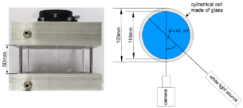
Figure 1. Cylindrical glass cell between two aluminium plates (left) and a sketch of the top view of the experimental setup (right), showing the crucial angle between the white light sheet for the illumination of the TLCs and the observation by a color camera.
Download figure:
Standard image High-resolution imageFor the investigation of the correlation between the color signal of the TLCs and their temperature, calibration measurements were carried out within a temperature range from T = 17 °C to T = 40 °C. In order to avoid a systematic uncertainty due to local temperature variations within the cell, about 20 min have been waited between each working point to obtain isothermal conditions during the measurements. Furthermore, a stirrer was circulating the water in the cell within those 20 min for ensuring the temperature uniformity. The side wall made of glass, which is a poor heat conducting material, is not expected to have any disturbing effects on the isothermal state in the cell. Therefore, this experimental setup is ideally suited for investigating the color signal of TLCs in dependency of the temperature and observation angle. The latter was varied from  to
to  in steps of
  by changing the direction of the light sheet relative to the fixed camera axis, shown on the right side of figure 1. Fifty images of the color signal were recorded with a frequency of
  for each observation angle and temperature. For the current study, the TLCs were not exposed to temperatures, which are considerably beyond their nominal range, as this would affect the correlation between color and temperature due to hysteresis [25] or even irreversible damages of the crystalline texture.
In order to investigate the influence of the illumination spectrum on the color appearance of TLCs, the SPECTRA X light engine (Lumencor, Inc.) was used as a light source [19]. This light source offers the possibility to adapt the wavelength spectrum, as it contains six solid-state LED light sources (violet, blue, cyan, green, red and near-infrared) emitting different color bands across the visible spectrum with tunable intensity. Two different wavelength spectrums for the illumination of the TLCs were used, which are depicted in figure 2. The first spectrum shows the case that all LEDs were switched on and, except for the green LED with a central wavelength of about  nm, were operated at maximum intensity. The power of the green LED was set to 50% of the maximum, due to its high power compared to the other ones. For the second spectrum the intensity of the blue LED was set to 40%, the cyan LED to 30%, the green LED to 40% and the red LED to 100% of the respective maximum. Furthermore, the violet and near-infrared LED were switched off, as the color camera is mainly sensitive from
  nm to
nm to  nm.
nm.
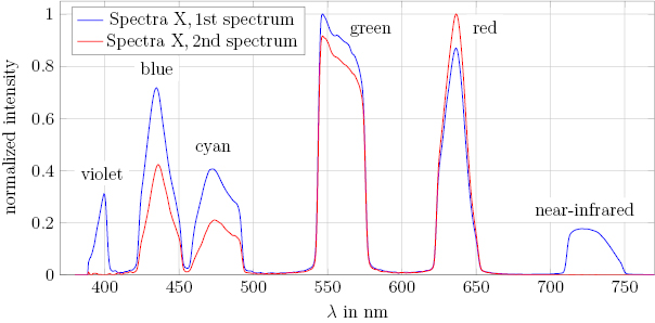
Figure 2. Spectrums for the illuminations of the TLCs R20C20W.
Download figure:
Standard image High-resolution imageIn addition, aside from the investigations of the color appearance of TLCs in the isothermal state, presented in section 3, this experimental setup enables one to induce thermal convection, when the cell is heated from below and cooled from above. The characteristic flow structures, which arise from differences of the fluid's density, are predestinated to demonstrate the possibility to measure velocity and temperature fields with TLCs simultaneously, presented in section 4.
3. Results
In order to illustrate the dependency of the color appearance of the TLCs on the temperature, three images of the TLCs in the cell for three different temperatures, applying an observation angle of  , are depicted in figure 3. These images clearly show the change of the color from red to blue with increasing temperature. However, in contrast to the specifications of the TLCs R20C20W, given by the manufacturer for an observation angle of
  , the TLCs already appear blue at a temperature of about T = 21 °C.
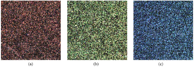
Figure 3. Color appearance of the TLCs R20C20W for different temperatures and an observation angle of  . The images show central sections of the cylindrical cell with dimensions of about
  . (a) T = 18.5 °C. (b) T = 19.0 °C. (c) T = 21.0 °C.
Download figure:
Standard image High-resolution imageFigure 4 shows the TLCs in the whole cell at T = 19 °C and  . The strong color play from the left to right end of the cell indicates that the actual observation angle changes locally from left to right due to refraction at the cylindrical wall of the cell. In order to limit variations of the observation angle inside the evaluated area, only a small section in the center of the cell was chosen, because the adjusted observation angle
  only applies to the center of the cell. This area, which is marked in figure 4, reaches over 100 px in the horizontal and 600 px in the vertical direction, yielding a negligible change of the color within this area at constant temperature. Therefore, all the investigations of the color appearance of the TLCs R20C20W in dependency of the temperature for different observation angles as well as the two illumination spectrums refer to this central section of the cell, which corresponds to dimensions of about
  .
.
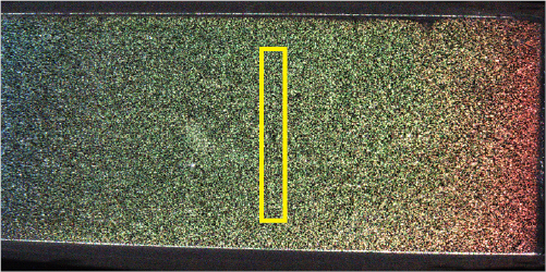
Figure 4. Snapshot of the TLCs R20C20W for T = 19 °C and an observation angle of  . The yellow rectangle indicates the section for evaluation.
Download figure:
Standard image High-resolution imageFor the characterization of the color of the TLCs in this small section, the red, green and blue intensities of each pixel, given by the internal algorithm of the camera, were extracted and transformed to the  -colorspace with its three quantities hue (H), saturation (S) and value (
 ) [26]. Using this colorspace, hue gives the shade of the color in terms of an angle in the range
 ![$\in [0^{\circ},360^{\circ}]$](https://content.cld.iop.org/journals/0957-0233/30/8/084006/revision2/mstab173fieqn023.gif) , which starts with red at
, which starts with red at  , passes green at
  , blue at
  and reaches red again at
  . In the following, hue is normalized with
  , so that
 ![$H \in [0,1]$](https://content.cld.iop.org/journals/0957-0233/30/8/084006/revision2/mstab173fieqn029.gif) . Furthermore, the saturation describes, if the color is rather pure (S = 1) or white (S = 0), while the value
. Furthermore, the saturation describes, if the color is rather pure (S = 1) or white (S = 0), while the value  represents the brightness of the color signal with
 ![$V \in [0,1]$](https://content.cld.iop.org/journals/0957-0233/30/8/084006/revision2/mstab173fieqn031.gif) . For a reliable evaluation, the mean values of hue, saturation and value were determined over all 50 images and over the whole section marked in figure 4 for each observation angle and temperature, respectively. The mean value of hue
. For a reliable evaluation, the mean values of hue, saturation and value were determined over all 50 images and over the whole section marked in figure 4 for each observation angle and temperature, respectively. The mean value of hue  over the marked area A and time t is depicted in figure 5 for both spectrums of illumination. It is emphasized, that the value of hue must be unambiguously correlated to the temperature for reliable temperature measurements. According to this condition, the following investigations refer to the temperature range from the minimum of each curve towards higher temperatures.
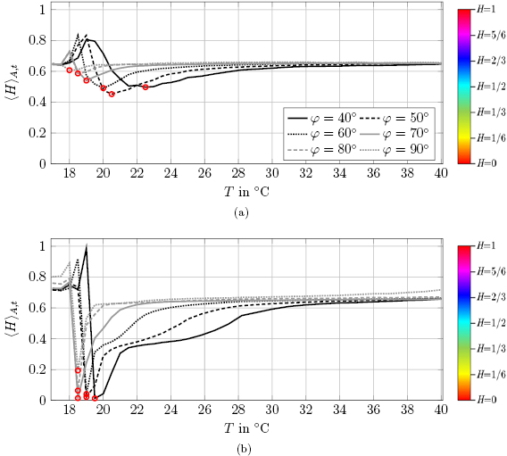
Figure 5. Color appearance of the TLCs R20C20W in dependency of the temperature for different observation angles applying the 1st spectrum (a) and 2nd spectrum (b) of illumination. The observation angles are given in the legend and are valid for both subfigures. For a better illustration, the colorbar on the right side shows the change of color appearance with hue. The red markers at the minimum of each curve indicate the onset of the investigated temperature range with unambiguous correlation to the color appearance of TLCs in terms of hue, respectively.
Download figure:
Standard image High-resolution imageAt first, it can be seen that the color appearance of the TLCs varies much more significantly for the second spectrum in figure 5(b). Considering only the temperature range from the minimum of each curve towards higher temperatures, hue mostly starts between H = 0 and H = 0.1 and reaches up to approximately H = 0.7. This corresponds to a change of color from red to blue with increasing temperatures. Concerning the influence of the observation angle, the color of TLCs in terms of hue changes faster for low temperatures, but remains nearly constant for higher temperatures, if larger angles are used. Therefore, the fast change of color at the lower end of the temperature range for large observation angles, which has already been discussed for  based on figure 3, is confirmed. On the contrary, there is still a stronger change of color for higher temperatures when smaller observation angles are applied. Moreover, the hue curves shift slightly towards lower temperatures with an increasing observation angle, meaning that the unambiguous temperature measurement range already starts at lower temperatures.
In comparison, hue varies only to a smaller extent when using the first spectrum of illumination. In this case, the largest dynamic range for hue is obtained for  , varying from about H = 0.45 to H = 0.65 in the temperature range from the minimal hue value towards higher temperatures. For all the other observation angles, the value of hue is also within this range, showing that the light reflected by the TLCs is more blue due to a higher intensity of the illumination in the blue wavelength range. Hence, the second spectrum is better suited for the illumination of the TLCs, as they show a significantly stronger color play with temperature. In order to use an appropriate observation angle for the illumination of the TLCs, it is important to estimate the effect of the observation angle on the uncertainty of measurement. Therefore, hue was investigated in the temperature range between T = 18.5 °C and T = 25 °C for using the second spectrum of illumination, as the slope of hue with temperature shows the largest differences in this range. For example, strong changes of hue are present in this range, when applying an observation angle of
  , while the slope of hue with temperature is mostly flat for
  or
or  . This allows to draw conclusions about the influence of the slope of hue on the uncertainty of temperature measurement. For this, the standard deviation of the mean value of hue
  over the whole evaluated section was calculated for the fifty images at each temperature step, as this quantity is directly related to the uncertainty of the temperature measurement. The resulting standard deviation of temperature
  can be estimated according to equation (1).

In order to determine the local slope of the calibration curve at each temperature set for the calibration measurements, the central difference quotient is used for linearization. Hence, the standard deviation of temperature is calculated according to equation (2), where the index i refers to the temperatures set for the calibration measurements. For a better illustration, the principle of the calculation is shown in figure 6.
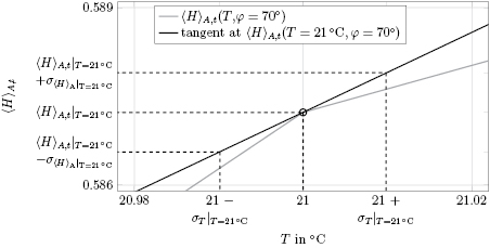
Figure 6. Influence of the standard deviation of hue on the standard deviation of temperature using the central difference quotient for linearization around the working point at the example of T = 21 °C and  .
.
Download figure:
Standard image High-resolution imageThe resulting standard deviation of hue and of the temperature are depicted in figure 7. Both quantities are shown in logarithmic scale to cope with their large change over two orders of magnitude. It has to be noted, that the results for  ,
,  and
and  are not plotted for the lowest temperatures, since the minimal hue value and, therefore, the onset of the temperature range with unambiguous correlation to the color appearance of TLCs is at higher temperatures. The standard deviation of the hue value reveals the trend to decrease with increasing temperature, as the hue value changes to less extent at higher temperatures, see figure 5. However, figure 7(b) shows that
  increases with temperature in most cases despite the decreasing standard deviation of the hue value. This is due to the fact, that steep gradients of hue with temperature at the lower end of the shown temperature range reduce the effect of larger standard deviations of hue, according to equation (2). For instance, applying an observation angle of
  a standard deviation of hue at T = 19 °C of about
  leads to a standard deviation of temperature of about
  K. In comparison, the standard deviation of hue at T = 25 °C for
  , which is approximately
  and thus much smaller, leads to a significantly larger standard deviation of temperature of about
  K. Furthermore, it can be seen that
  increases faster for larger observation angles. While the minimum for the mean value of
  within the temperature range from T = 18.5 °C to T = 25 °C is obtained for
  with approximately
  K, the mean value of
  amounts to about
  K for
K for  . Hence, increasing the observation angle allows for precise temperature measurements in a decreased range. In summary, figure 7 shows the considerable influence of the local slope of
  on the uncertainty of temperature measurement, which increases with decreasing slope. This slope strongly depends on the observation angle, which must therefore be chosen advisedly. According to figure 7(b), the observation angles
  ,
,  and
and  are most applicable for precise temperature measurements, which is why the following investigations are restricted to those three angles.
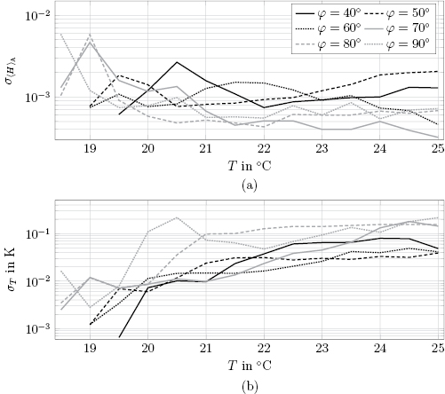
Figure 7. Standard deviation of the spatial mean value of hue  in the evaluated section according to figure 4 in dependency of the temperature for different observation angles (top) and the resulting standard deviation of the calculated temperatures (bottom). The observation angles are given in the legend and are valid for both subfigures. (a) Standard deviation of hue. (b) Standard deviation of temperature.
Download figure:
Standard image High-resolution imageBesides hue  , also the saturation
  and value
  might give some additional information for the determination of the temperature. In order to estimate their usability, these quantities are depicted in figure 8, depending on the temperature for
  ,
,  and
and  . It can be seen that there is no explicit correlation of the saturation or value to the temperature, which could be of great advantage for the calibration of the temperature measurement. This is partly due to the experimental conditions, as for example a varying seeding concentration. In comparison,
  is not sensitive to the preparation of the suspension in terms of the seeding concentration or particle size and further parameters like the intensity of illumination. Therefore, only
  is taken into account for the calibration of the temperature measurements. This offers the possibility to calculate the temperature precisely via linear interpolation of
  , if the distance between the sampling points is sufficiently small.
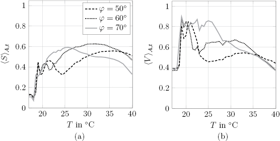
Figure 8. Mean saturation  and value
  of the TLCs R20C20W in dependency of the temperature for different observation angles applying the second spectrum of illumination. The observation angles are given in the legend and are valid for both subfigures. (a) Saturation S. (b) Value
  .
.
Download figure:
Standard image High-resolution imageAs already illustrated in figure 4, the color of the TLCs can also vary significantly inside the field of view even for a constant temperature, due to different observation angles. This has to be considered in the calibration. For that reason, the whole field of view has to be split into small interrogation windows, in order to obtain a local calibration curve  for each interrogation window. Hence, local variations of the color play due to different observation angles are taken into account. Here, the size of the interrogation windows was set to 64
  64 px. Figure 9 shows an exemplary calibration curve
  for an interrogation window in the center of the cell at
  as well as its post-processing aiming for an unambiguous correlation
  over the whole temperature range. This includes that the highest values of hue at low temperatures are reduced by one, leading to negative values of hue, but keeping the same color shade due to its cyclic definition. Furthermore, the post-processing has the effect that sampling points, which lead to a decrease of hue with increasing temperature, are ignored, resulting in an unambiguous correlation
  . Using this calibration approach for each interrogation window and linear interpolation between the sampling points for the calculation of the temperatures
  , low standard deviations in the range of
  K or even less can be achieved for
  ,
,  and
and  .
.
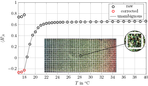
Figure 9. Postprocessing of an exemplary calibration curve of hue  for one interrogation window when using a two-dimensional (2D) calibration approach.
Download figure:
Standard image High-resolution imageFor a better illustration, figure 10 shows how a temperature field is calculated on the basis of an instantaneous snapshot of the calibration measurement at T = 19 °C and  , compare figure 4. In the first step, the hue field is computed based on the mean values of the red, green and blue intensities according to the equations in [26] for each interrogation window, which is depicted in figure 10(a). This hue field clearly demonstrates the need for a 2D calibration approach for the temperature measurement, because hue varies from about H = 0 at the right to about H = 0.5 at the left end, although there is a constant temperature of T = 19 °C. Determining the temperatures via linear interpolation of hue in each interrogation window with the corresponding calibration curve leads to the temperature field depicted in figure 10(b). It can be seen that the main part of the calculated temperatures is very close to T = 19 °C, yielding a standard deviation of about 0.04 K for this instantaneous temperature field, which demonstrates the low uncertainty of the temperature measurement using the calibration approach described above.
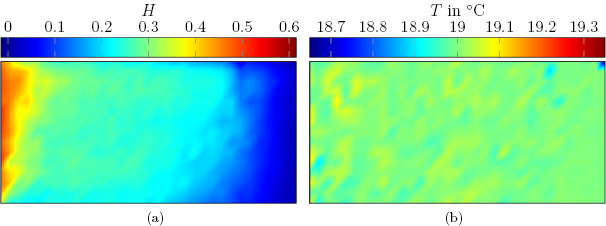
Figure 10. Hue field (left) and the corresponding calculated temperature field (right) for an exemplary snapshot of the TLCs R20C20W at homogeneous temperature of T = 19 °C in the whole cell and an observation angle of  in the center, see figure 4. (a) Hue field. (b) Corresponding calculated temperature field.
Download figure:
Standard image High-resolution imageIn order to compare the quality of this calibration approach for different temperatures and observation angles, figure 11 shows the mean deviation of the calculated temperatures to the set values of temperature for  ,
,  and
and  , considering all of the 50 images for each temperature step, respectively. Furthermore, the standard deviation of the calculated temperatures is shown as an error bar for each temperature step. In order to be consistent with the previous investigations, the results refer to the section in the center of the field of view, which is marked in figure 4.
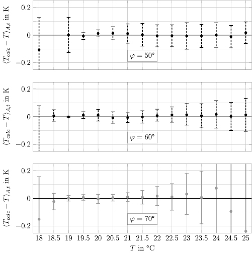
Figure 11. Mean deviation of the calculated temperatures to the set value of temperature with error bars showing the standard deviation of the calculated temperatures for  (top),
  (center) and
  (bottom) using the second spectrum of illumination.
Download figure:
Standard image High-resolution imageAs already shown above, the temperature range from T = 18.5 °C to T = 25 °C is most applicable for precise temperature measurements, due to the largest gradients of hue with temperature, see figure 5. Therefore, the results in figure 11 are mainly restricted to this temperature range, but slightly extended to lower temperatures, as the calibration approach according to figure 9 ensures an unambiguous correlation between hue and temperature. It has to be noted that the error bar for  and T = 18.5 °C can not be seen due to a higher deviation to the set value of temperature, which amounts to about
  K. As can be seen in figure 11, larger observation angles are better suited for temperature measurements in the lower end of the shown temperature range. Especially, in the range from T = 18 °C to T = 19 °C only the observation angle
  proves to be suitable, as no outliers regarding the mean deviation of the calculated temperatures to the set value of temperature and the standard deviation of temperature occur. This is due to the fact, that the unambiguous correlation between hue and temperature already starts at lower temperatures without any post-processing steps when applying larger observation angles, see figure 5. For temperatures between T = 19 °C and T = 22.5 °C the best results are obtained for all three observation angles. In this range, the mean deviation of the calculated temperatures to the set value of temperature is in between
  K for each observation angle. Furthermore, the standard deviation does not exceed
  K, with exception from T = 19 °C applying an observation angle of
  . It can further be seen that the mean deviation as well as the standard deviation increases considerably for T > 23.5 °C when using an observation angle of
  . This can be explained by the the fact that the color signal only changes to less extent for
  when increasing the temperature to T > 23.5 °C. Therefore, an observation angle of
  or even larger is not suited for measuring temperatures larger than T = 23.5 °C, when the TLCs R20C20W are used.
4. Application
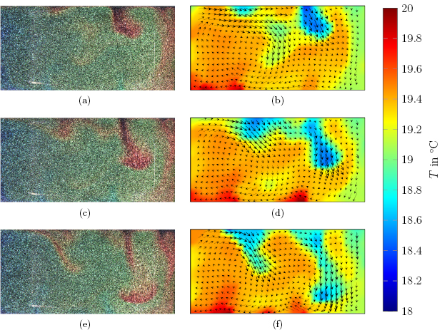
In order to demonstrate simultaneous measurements of velocity and temperature fields, the setup was used as a Rayleigh–Bénard system. For this, the bottom plate was heated up to a constant temperature of T = 21 °C, while the top plate was cooled down to T = 18 °C using another temperature control unit, inducing thermal convection due to the variation of the fluid's density caused by the temperature gradient between bottom and top plate. An observation angle of  was used as it promises low uncertainty of temperature measurement for the occurring temperatures between T = 18 °C and
  , while keeping perspective errors within reasonable limits. In figure 12 three instantaneous image captures of the TLCs with a time gap of two seconds can be seen on the left-hand side. These images clearly show the motion of convective flow patterns, in particular a cold plume at the top of the cell, represented by red colored TLCs, sliding down within this time span due to a higher density. The right column of figure 12 shows the corresponding temperature fields calculated on the basis of a 2D calibration as described above, using interrogation windows with a size of 64
  64 px. Compared to the image captures of the TLCs on the left side, the temperature of the flow structures can be reproduced successfully. In addition, the superimposed velocity vectors determined with a planar PIV-algorithm [9, 10] indicate the motion of the fluid according to the local temperature correctly. Since this application of TLCs is presented to show the possibility of simultaneous velocity and temperature field measurements, further investigations about Rayleigh–Bénard convection itself are not addressed here. However, as the evolving flow structures in Rayleigh–Bénard convection are of paramount interest, it is referred to [4] and [5] for detailed analysis.
Figure 12. Three exemplary images of the TLCs R20C20W with a time gap of two seconds in Rayleigh–Bénard convection with a heating plate temperature of T = 21 °C and cooling plate temperature of T = 18 °C (left) as well as the corresponding fields of velocity and temperature (right). (a) Image of TLCs R20C20W, t = 0 s. (b) Velocity and temperature field, t = 0 s. (c) Image of TLCs R20C20W, t = 2 s. (d) Velocity and temperature field, t = 2 s. (e) Image of TLCs R20C20W, t = 4 s. (f) Velocity and temperature field, t = 4 s.
Download figure:
Standard image High-resolution image
5. Conclusion
In order to perform precise temperature measurements using TLCs, a strong color variation with temperature is of advantage, which depends on the spectrum of the white light source needed for the illumination and the observation angle. In this work, the color signal of the TLCs of type R20C20W (LCR Hallcrest) was investigated for two different spectrums of illumination. In addition, different observation angles, ranging from  to
to  , were applied. While there is only a slight change of the color of TLCs with temperature for the first spectrum, the second spectrum with an increased intensity of red light and decreased intensity of blue light leads to a larger range of color play of the TLCs, covering nearly the whole visible spectrum. One main result obtained by the investigations concerning the observation angle is that the color of TLCs changes faster with temperature at the lower end of the temperature range of color play, if the observation angle is increased. However, the change of color with temperature decreases very fast for larger observation angles. Since the investigations have shown, that strong color changes are advantageous for a low uncertainty of temperature measurement, it can be concluded that larger observation angles enable precise temperature measurements at the expense of a smaller measurement range. On the contrary, applying smaller observation angles allows for temperature measurements over a larger temperature range, which is extended to higher temperatures, while the uncertainty of the temperature measurement at the lower end of the range increases. Hence, depending on the application, the observation angle offers the possibility to be adapted to the temperature range of interest using the same type of TLCs, so that preferably strong color variations exist over the desired measurement range. Furthermore, observation angles in the range from
  to
to  lead to the lowest standard deviations of the temperature measurement. Particularly in the temperature range from T = 18.5 °C to T = 25 °C, standard deviations in the range of 0.1 K or even less were achieved. However, in contrast to the temperature measurements, an observation angle of
  is of advantage for simultaneous velocity measurements with PIV, tracing the TLCs with the same color camera. In order to overcome this issue, two cameras can be used. While a color camera placed at an observation angle between
  and
and  is used to determine the temperature distribution, the velocity of the TLCs can be measured via another camera, applying a standard PIV configuration with perpendicular detection. Another advantage of this setup is the possibility to adjust the exposure time to optimal results for both cameras, since for the determination of the temperature slight motion blur can be accepted with regard to a high signal-to-noise ratio (SNR), contrary to the velocity measurements using PIV. In this way, the combination of PIV and PIT using TLCs offers the possibility to measure velocity and temperature fields simultaneously with unique accuracy.
Acknowledgments
The authors are very grateful to Alexander Thieme for the technical support and to Theo Käufer for the assistance during the measurements.