


Abstract
A detailed interpretation of scanning tunneling spectra obtained on unconventional superconductors enables one to gain information on the pairing boson. Decisive for this approach are inelastic tunneling events. Due to the lack of momentum conservation in tunneling from or to the sharp tip, those are enhanced in the geometry of a scanning tunneling microscope compared to planar tunnel junctions. This work extends the method of obtaining the bosonic excitation spectrum by deconvolution from tunneling spectra to nodal d-wave superconductors. In particular, scanning tunneling spectra of slightly underdoped  with a
  of 82 K and optimally doped
  with a Tc of 92 K reveal a resonance mode in their bosonic excitation spectrum at
  and
and  respectively. In both cases, the overall shape of the bosonic excitation spectrum is indicative of predominant spin scattering with a resonant mode at
  and overdamped spin fluctuations for energies larger than 2Δ. To perform the deconvolution of the experimental data, we implemented an efficient iterative algorithm that significantly enhances the reliability of our analysis.
Export citation and abstract BibTeX RIS

Original content from this work may be used under the terms of the Creative Commons Attribution 4.0 license. Any further distribution of this work must maintain attribution to the author(s) and the title of the work, journal citation and DOI.
1. Introduction
With the intention to unravel the unconventional pairing mechanism in high-temperature superconductors, extensive effort has been put into extracting the spectral density of the pairing boson from experimental data [1–10]. An ever-present contender for this 'bosonic glue' are antiferromagnetic spin fluctuations which have been extensively studied in the family of cuprate superconductors [11–15]. Such an electronic pairing mechanism leads to a heavy renormalization of the boson spectrum when entering the superconducting state. In the normal state, overdamped spin excitations form a broad and gapless continuum. In the superconducting state, they develop a spin gap of 2Δ, the minimum energy needed to create a particle-hole excitation, plus a rather long-lived resonance mode at  inside the spin gap [16–26]. This resonance is made possible by the sign-changing (d-wave) symmetry of the superconducting gap and identified as a spin exciton [18]. The above mentioned behavior of the spin excitation spectrum has been directly observed in inelastic neutron scattering (INS) experiments [11, 12, 27–31] yielding strong evidence for spin-fluctuation mediated pairing. Since signatures of this resonance mode are also expected to be visible in optical, photoemission and tunneling spectra, a considerable number of studies tried to complete the picture using these techniques [2–9, 32–36], all probing a slightly different boson spectrum and facing complicated inversion techniques. Recently, machine learning algorithms entered the scene and their application to angle-resolved photoemission (ARPES) data proved to be a powerful concept to reverse-model the spin-spectrum, but this happens at the cost of a number of free parameters which cannot be easily mapped onto physical quantities [10, 34]. In this work, we extracted the bosonic spectrum from the inelastic part of scanning tunneling spectra which we obtained on the cuprate superconductors
  (Bi2212) and
  (Y123). In contrast to previous scanning tunneling spectroscopy (STS) [3, 35] and break junction experiments [37] that focused on Bi2212, we obtain the boson spectrum without a functional prescription and over a wide energy range for both materials. It naturally exhibits the sharp resonance mode and overdamped continuum that are characteristic for the spin spectrum measured in INS.
Inelastic electron tunneling spectroscopy experiments using the tip of a scanning tunneling microscope (IETS-STM) have proven to be a powerful tool in the study of bosonic excitations of vibrational [5, 38–41], magnetic [42–47] or plasmonic [38, 48] character in metals, single molecules and also superconductors. Due to the spatial confinement of the electrons in the apex of the STM tip, the wave vector of the tunneling electrons is widely spread and the local density of states (LDOS) of the tip becomes rather flat and featureless. Consequently, the generally momentum dependent tunnel matrix element can be considered momentum independent in the STM geometry [49]. As a result, the elastic contribution to the tunneling conductance  becomes directly proportional to the LDOS of the sample at the tip position, as has been shown by Tersoff and Hamann [50], which makes STM a surface sensitive technique similar to planar tunneling junctions or photo emission spectroscopy. In the context of cuprates, this means that all these techniques study superconductivity near the surface. The inelastic contribution
  to the tunneling conductance is given by a momentum integrated scattering probability of tunneling electrons sharing their initial state energy with a final state electron and a bosonic excitation. The absence of strict momentum conservation opens the phase space for the excited boson and as a consequence, the inelastic contributions to the tunneling current can be a magnitude larger than in planar junctions [41], in which the lateral momentum is conserved.
Previous IETS-STM experiments used this effect to determine the Eliashberg function  of the strong-coupling conventional superconductor Pb [41, 51], which contains the momentum integrated spectral density of the pairing phonon
  , as well as the electron–phonon coupling constant
  [52–54]. While for conventional superconductors, the Migdal theorem [55] allows to treat the electronic and phononic degrees of freedom to lowest order separately, largely simplifying the analysis of IETS spectra, the situation is less clear for unconventional superconductors with electronic pairing mechanism. Nevertheless, the theoretical description of IETS-STM spectra could be extended to the fully gapped Fe-based unconventional superconductors of
  character [56, 57]. Strong coupling of electrons and spin fluctuations manifests in IETS-STM spectra as a characteristically lower differential conductance in the superconducting state compared to the normal state for energies slightly below 3Δ [56]. Also for these systems, the boson spectrum could be reconstructed from IETS-STM spectra by deconvolution [57]. In this work, we investigate, in how far this method can be extended to nodal d-wave superconductors. To do this, we follow the path of a deconvolution of scanning tunneling data, using a priori band structure for the normal state model and the inelastic scanning tunneling theory of unconventional superconductors derived by Hlobil et al [56].
2. Methods
2.1. Outline of the extraction procedure
The total tunneling conductance  between a normal conducting tip and a superconductor is comprised of the elastic tunneling contributions
  , but also significant inelastic contributions
  [41, 51, 56, 57]. While the second derivative of the tunneling current
  obtained on conventional superconductors in the normal state is directly proportional to the Eliashberg function
  [51], the bosonic glue in unconventional superconductors is drastically renormalized upon entering the superconducting phase.
In the presence of strong inelastic contributions to the tunneling current an inversion procedure á la McMillan and Rowell [52] cannot be used to extract the Eliashberg function from the superconducting spectrum. As was shown in [56], the function  acts as the 'generalized glue function' and analog to the Eliashberg function in superconductors driven by electronic interactions. As both, phonons and spin fluctuations, may couple to the tunneling quasiparticles, we define the bosonic spectrum

where g is the spin-fermion coupling constant and  is the dimensionless, momentum integrated spin spectrum. The inelastic differential conductance for positive voltage at zero temperature is given by

While the explicit momentum dependence of the bosonic spectrum is lost in this form, it still contains the spin resonance at the antiferromagnetic ordering vector if antinodal points on the Fermi surface contribute significantly to the tunneling spectrum. As can be seen from equation (2), B is the source function, the density of states (DOS) in the superconducting state νs
is the kernel and the inelastic tunneling conductance  is the signal. Θ denotes the Heaviside step function. The general aim in this work is to extract the function
  as accurately as we can from scanning tunneling spectra, which we do by deconvolution of equation (2). We follow the following step-by-step procedure:
- 1.Determination of the superconducting density of states νs
- 2.Determination of the inelastic tunneling conductance

- 3.Extraction of by deconvolution of equation (2)


Assumptions and limitations of our extraction procedure are discussed in section 2.1.4.
2.1.1. Step 1: Determining νs .
From a scanning tunneling spectrum below Tc
we obtain the differential conductance d d
d . This function consists of the purely elastic part
  and the inelastic part
  . The elastic part is directly proportional to the superconducting density of states in the sample νs
. In this step, we determine the functional form of the elastic contribution by fitting a model function to the low bias region of the d
. The elastic part is directly proportional to the superconducting density of states in the sample νs
. In this step, we determine the functional form of the elastic contribution by fitting a model function to the low bias region of the d dU spectrum that keeps the complexity as low as possible while still capturing the relevant features of the band structure and pairing strength. We opt for a generalized Dynes function [58] with a momentum dependent gap:

Here,  is a normalization factor,
  is the d-wave pairing potential,
  the quasiparticle scattering rate,
  is the angle-dependent DOS at the Fermi energy in the normal conducting phase, λ the band index and Cλ
the relative tunneling sensitivity for the band. The function
is the angle-dependent DOS at the Fermi energy in the normal conducting phase, λ the band index and Cλ
the relative tunneling sensitivity for the band. The function  weighs gap distributions for different
  by their abundance along the Fermi surface (FS). It is derived from a microscopic tight-binding approach that models the dispersion relation. In the case of Bi2212 we used a single-band model whereas for Y123 we considered two CuO2 plane bands and one CuO chain band (see appendix
  has a nodal structure. This prevents us from directly assigning the differential conductance for
  to the purely elastic tunneling contribution as was possible for the
  superconductor monolayer FeSe [56, 57]. We will, however, start from here and refine
  in the next step.
2.1.2. Step 2: Determining .

We use the fact that  and the physical constraints
  and
and  . In order to relate our fitted curve to
  , we need to make an initial guess for
  in the range
  . As a first guess, we assume
  to be directly proportional to
  . This is equivalent to assuming that
  and we can rewrite for that energy regime:

In fact, we rather expect  to be a slowly increasing function with a soft spin gap for
  due to the ungapped parts of the Fermi surface, but our choice of
  is only a first guess and will later be refined. Additionally, the delta distribution at zero is far away from the physically interesting energy regime, which avoids a misinterpretation of the final extracted boson spectrum. The introduction of the numerical scaling factor η is also necessary from a computational standpoint as it can ensure that
  and
and  are always positive, which is a prerequisite for our extraction procedure. We approximated η using a boundary condition for the total number of states (see appendix
  (D denotes the energy scale of the band edge), we scale up our experimental curve by
  instead of scaling down our fitted curve.
  is then simply the difference of the scaled up (by
  ) experimental data points and the Dynes fit (
 ). We took care that the choice of this numerical factor, that simply helps to perform our deconvolution algorithm and paint a more realistic picture of
  , does not influence the extracted boson spectrum in a qualitative manner (see appendix
2.1.3. Step 3: Extracting .

We compare two methods by which the boson spectrum was determined: The direct deconvolution in Fourier space and the iterative Gold algorithm [59, 60] to perform the deconvolution. The advantage of the Gold algorithm is that for positive kernel and signal, the result of this deconvolution method is always positive. This is in agreement with our physical constraint that the bosonic excitation spectrum is strictly positive. We used the implementation of the one-fold Gold algorithm in the TSpectrum class of ROOT system [61, 62] in C language wrapped in a small python module.
The bosonic function from direct deconvolution in Fourier space is obtained from

where  denotes a Fourier Transform and
  the inverse transform. The abrupt change in elastic conductance at zero energy (multiplication with Heaviside distribution in equation (2)) leads to heavy oscillations in the Fourier components. Therefore the result of this deconvolution procedure can contain non-zero contributions for E < 0 and negative contributions for
  . They are exact solutions to equation (2) but from a subset of non-physical solutions that we are not interested in. Because the solutions obtained in this way are highly oscillatory we show the result after Gaussian smoothing. In order to obtain a positive solution to equation (2), the result of the direct deconvolution method is used as a first guess to the Gold algorithm. The results shown in this work are obtained after 2000 000 iterations at which point convergence has been reached.
2.1.4. Assumptions and limitations.
In order for our extraction method to be applicable, several simplifying assumptions were made:
- 1.Quasiparticles with energy ω couple to bosonic excitations of energy Ω and effective integrated density of states. The k-dependence of the interaction is thus disregarded.
- 2. has a simple relation to for (see section 2.1.2) which is generally oversimplified for d-wave superconductors, especially near Δ.


In general, retrieving the source function from a convolution integral is an ill-posed problem which means that we only obtain one solution from a large set of valid solutions to the convolution equation. Additional aspects that complicate the problem are the following:
- 1.The kernel function is a guess which is very dependent on the modeling of the superconducting density of states and is further questioned by lack of energetic regions of purely elastic processes in the scanning tunneling spectrum. We are in fact on the verge of a necessity for blind deconvolution algorithms.
- 2.Strong electron-boson coupling leads to spectral features of outside the gap [52, 63, 64] that are neglected here as the contribution of is expected to be much larger. They can in principle be reconstructed within an Eliashberg theory using the extracted boson spectrum. Using this refined and repeating the procedure until leads to the correct and could further improve our result.
- 3.Electronic noise in the recorded spectra is ignored and consequently ends up in either νs or.
- 4.With we obtain only an 'effective tunnel Eliashberg function' which includes all bosonic excitations that are accessible to the tunneling quasiparticles. Hence, no disentanglement into lattice and spin degrees of freedom is possible.
- 5.The k-dependence of is inaccessible.


2.2. Experimental methods
We performed inelastic tunneling spectroscopy on a slightly underdoped Bi2212 sample with a Tc
of 82 K (UD82) and an optimally doped Y123 sample with a Tc
of 92 K (OP92) using a home-built STM with Joule-Thomson cooling [65]. The samples were cleaved at a temperature of 78 K in ultra-high vacuum (UHV) and immediately transferred into the STM. Successful cleaving was determined by optical inspection with a telescope as well as low surface roughness and a clear superconducting gap in STM. All spectra were recorded with a tungsten tip. The tungsten tip was electrochemically etched in air and then directly transferred into a UHV chamber, where it was ion etched with keV Ar+ ions and flashed to high temperatures above the melting point in order to remove oxides and carbides. To rule out unwanted effects of a non-flat tip DOS, it was characterized on a Cu(111) surface before turning to the cuprate. The set-up also allows to vary the temperature of the STM in order to record spectra above Tc
. Due to the large inhomogeneity of scanning tunneling spectra on Bi2212 [66], we show averaged spectra recorded at positions, where the dip-hump feature can be clearly seen. In the case of Y123, the overall spectral inhomogeneity was lower (see appendix  area where the dip-hump feature was ubiquitous.
3. Results and discussions
3.1. Bismuth strontium cuprate

3.1.1. Experimental results.
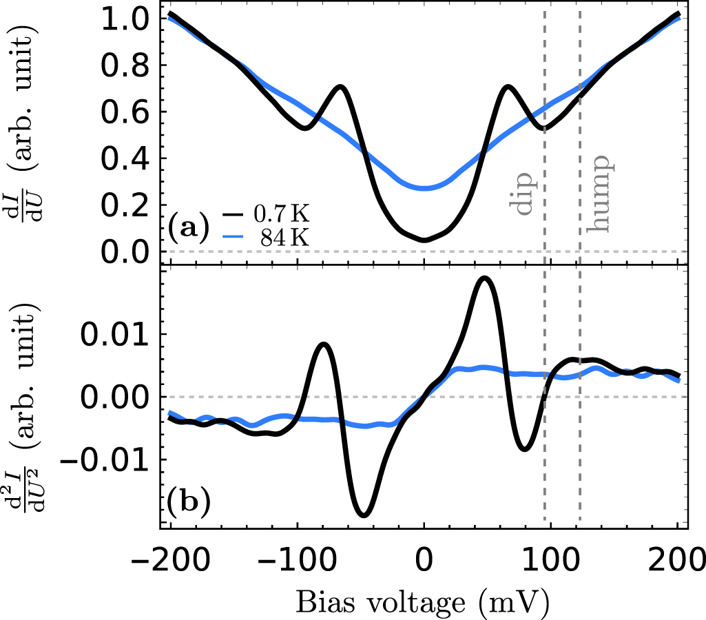
Figure 1 shows experimental  and
and  spectra recorded at 0.7 K and 84 K. In order to remove a linear background that stems from a slope in the DOS due to hole doping [67, 68] and prepare the data for further analysis of particle-hole symmetric features, we follow a previous work [57] and symmetrized the
  spectra in figure 1(a). This procedure does not affect the quasi-particle spectrum due to particle-hole symmetry of the superconducting state and the inelastic contribution to the tunneling current. The dI/dU spectrum for superconducting Bi2212 in figure 1(a) shows a single but smeared gap with residual zero-bias conductance due to the nodal
  gap symmetry. Similarly, the coherence peaks are smeared due to the gap symmetry and possibly also due to short quasiparticle lifetimes. This is typical for the underdoped regime and may be caused by its proximity to the insulating phase [66]. Outside the gap, a clear dip of the superconducting spectrum below the normal conducting spectrum, followed by a hump reapproaching it, are visible. The V-shaped conductance in the normal state hints towards strong inelastic contributions to the tunneling current from overdamped electronic excitations discussed in context of cuprates and iron-based superconductors in [56, 69, 70]. A similar V-shape due to inelastic scattering off phonons has even be reported for conventional superconductors like Pb [41]. In contrast to phonons, electronic excitations become partly gapped in the superconducting state causing a redistribution of the spectrum in form of dip-hump features in the differential conductance. The hump shows as a peak in the second derivative of the tunneling current that exceeds the curve of the normal state at
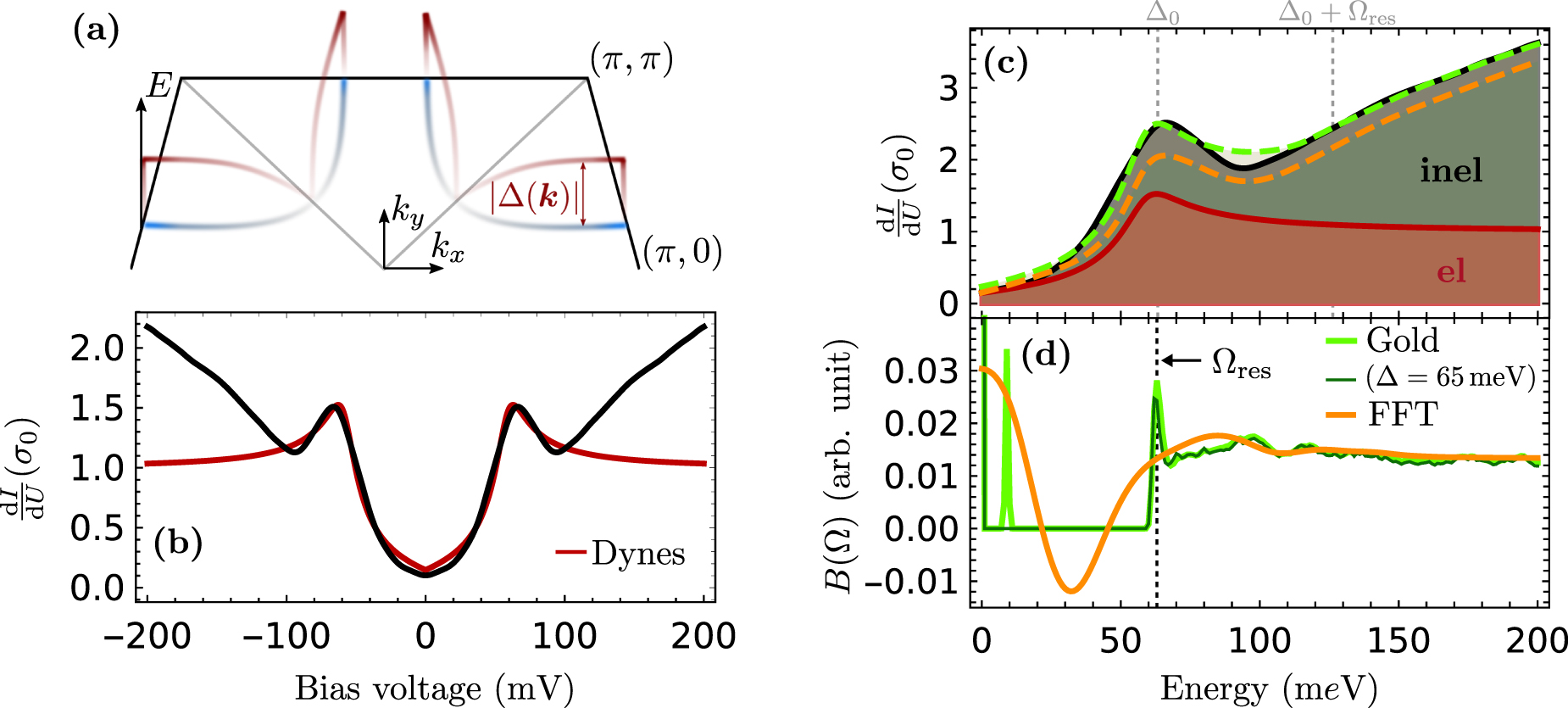
  in figure 1(b). The relatively round shape of the superconducting gap in Bi2212 is atypical for a classic d-wave superconductor, in which the naive expectation is a V-shaped conductance minimum. As will be shown later on, the round shape of the gap can be generated without admixture of an s-wave pairing term by respecting the anisotropy of the Fermi surface in the normal state. The Fermi surface and gap anisotropy are summarized schematically in figure 2(a).

Figure 1. Tunneling Spectra on Bi2212: (a) Experimental  spectra in the superconducting/normal state (black/blue) recorded at 0.7/84 K after Gaussian smoothing, symmetrization and normalization to the differential conductance in the normal state at 200 mV. (b) Numerical derivative of spectra in (a).
Download figure:
Standard image High-resolution image
Figure 2. Bosonic Spectrum Extraction for Bi2212: (a) Schematic perspective view of the Fermi surface (FS) in the first Brillouin zone (BZ) in the normal/superconducting state (blue/red) (adapted from [71]). The color lightness depicts the relative density of states: the higher the lightness, the lower the density of states. (b) A generalized Dynes model (equation (3)) with  and
and  (red) was fitted to the experimental differential conductance (black). (c) The total conductance (black line) has been scaled up by the factor
  . The inelastic part of the conductance (vertical width of grey area) is given by the difference between the total (black) and the elastic part (red) of the conductance. Forward convolved conductance with the obtained boson spectral functions from the direct FFT method/Gold algorithm are shown in orange/green dashed lines. (d) Boson spectral function determined by direct FFT method/Gold algorithm (orange/green). The thin dark green line shows the boson spectral function for a different Dynes fit than in (b), (c) with
  (not least square minimum). The result of the direct FFT method has been regularized for clarity. A clear resonance mode at
  is visible. Zero-energy contributions are an artifact from the scaling procedure.
Download figure:
Standard image High-resolution image3.1.2. Extraction of the bosonic spectrum.
We followed the step-by-step extraction procedure outlined in section 2.1 starting from the determination of the superconducting density of states νs
. The optimal Dynes fit to our experimental spectrum in the superconducting state is shown in figure 2(b) with  (
( and
and  ) and
) and  . The resulting (in)elastic contribution is shown in red(grey) in figure 2(c). Here, a numerical scaling factor of η = 0.6 was used. The value for Δ lies within the range of previously reported gap values on the Bi2212 surface [66], especially in the slightly underdoped regime, where variations of the local gap from the average gap tend to be larger [72].
The regularized bosonic function from direct deconvolution in Fourier space is shown in figure 2(d) in orange. The contributions at low energies are an artifact from the scaling with factor η. Despite our uncompromising simplifications, the bosonic spectrum recovers well the tendency of the total conductance in the forward convolution (figure 2(c) orange) and shows the expected behavior for coupling to spin degrees of freedom at medium and high energies, i.e. a resonance mode at  and approach of the normal state bosonic function B for
  [56], that, in contrast to the Eliashberg function in the case of phonon-mediated pairing, remains finite for energies well above 2Δ. While the long-lived resonance mode is associated with a spin resonance due to the sign-changing gap function, the broad high-energy tail of the bosonic spectrum is due to the coupling to overdamped spin fluctuations, or paramagnons [18]. Resonant inelastic x-ray scattering (RIXS) studies have shown that these paramagnons dominate the bosonic spectrum for energies larger than
  in several families of cuprates as almost all other contributors, e.g. phonons, lie lower in energy [73–76].
By application of the Gold algorithm we obtained the bosonic spectrum shown in green in figure 2(d). Again, the high value at E = 0 is a consequence of the scaling with factor η. We could get rid of negative contributions and find a bosonic function that recovers well the total conductance (figure 2(c) green), especially the dip-hump structure, and shows a very clear resonance at  . The sharp peak at
  is due to inadequacies of our elastic fit in the region of the coherence peak. It is e.g. not present in our analysis of Y123 (see section 3.2) and vanishes once we take an elastic DOS with a larger gap (here
  , not least-square minimum) as we show in the thin dark green line in figure 2(d). This is in contrast to the resonance at
  , which remains and only decreases slightly in energy for the fit with a larger gap. This behavior is expected according to the hump in the tunneling spectrum at
  .
.
The resonance mode extracted in this work is higher in energy than reported in INS experiments ( at the antiferromagnetic ordering vector) [12] and closer to the resonance determined by optical scattering (
 ) [32]. Due to the loss of momentum information in tunneling, the center of the resonance is expected to be shifted to higher energies compared to the INS results [56]. Due to the large inhomogeneity of Δ on the surface of Bi2212 [66], it is more instructive to compare the ratio
  to other works rather than the absolute value of
  . The ratio
  lies within the current range of error of
  by Yu et al [25]. In most other extraction methods of the bosonic mode energy, the normal state DOS is not respected, which is why, depending on the method, the Δ0 used there is most similar to what is here called
  or
or  .
.  is the largest gap value that contributes to the elastic conductance spectrum and
  the momentum averaged and DOS weighted gap.
3.2. Yttrium barium cuprate

3.2.1. Experimental results.
The symmetrized dI/dU spectrum for superconducting Y123 in figure 3(a) is qualitatively in excellent agreement with previous STM measurements [77–82] and shows three low-energy features: (i) a superconducting coherence peak at  that is sharper than in Bi2212, (ii) a high-energy shoulder of the coherence peak and (iii) a low-energy peak at
  . The high-energy shoulder as well as the sub-gap peak are believed to arise from the proximity-induced superconductivity in BaO planes and CuO chains [80, 83–85]. This would certainly account for the fact that these states are missing in the Bi-based compounds and that the sub-gap peak shows a direction-dependent dispersion in ARPES data [86, 87]. At energies larger than Δ, we again find a clear dip-hump feature, similar as in Bi2212. The hump lies at
  as can also be seen from the second derivative of the tunneling current in figure 3(b). The V-shaped background conductance in the high-energy regime of the superconducting spectrum is in agreement with the predicted inelastic contribution by magnetic scattering in the spin-fermion model [56, 69].

Figure 3. Bosonic Spectrum Extraction for Y123: (a) A generalized Dynes model (equation (3)) with  for the anti-bonding (AB),
  for the bonding (BB) and
  for the chain (CH
 ) band (red) was fitted to the symmetrized experimental differential conductance (black). (b) Numerical derivative of spectrum in (a). (c) The total conductance (black line) has been scaled up by the factor
  . The inelastic part of the conductance (vertical width of grey area) is given by the difference between the total (black) and the elastic part (red) of the conductance. Forward convolved conductance with the obtained boson spectral functions from the direct FFT method/Gold algorithm are shown in orange/green dashed lines. (d) Boson spectral function determined by direct FFT method/Gold algorithm (orange/green). The result of the direct FFT method has been regularized for clarity. A clear resonance mode at
  is visible. Zero-energy contributions are an artifact from the scaling procedure.
Download figure:
Standard image High-resolution image3.2.2. Extraction of the bosonic spectrum.
We proceeded as in the case for Bi2212, but incorporated the one-dimensional band from the CuO chains as well as the bonding and anti-bonding band from the CuO2 planes into the calculation of the normal state DOS to remodel the sub-gap peak and coherence peak shoulder in the estimated  of the superconducting state. The optimal Dynes fit with gaps
  for the anti-bonding (AB),
  for the bonding (BB) and
  for the chain band is shown in red in figure 3(a). Because vacuum-cleaved surfaces favor tunneling into states of the CuO chain plane [77, 80, 88], the sub-gap peak is pronounced and the contribution to the total DOS of the CH
 band is, in our analysis, roughly five times higher than for the AB and BB band. The size of
  is in good agreement with other scanning tunneling spectroscopy results spanning around 20 experiments, in which the extracted gap value lies between
  for optimally doped samples [66]. For comparison: From Raman spectra, Δ0, i.e. the gap in the antinodal direction, is frequently found to be
  for optimally doped Y123 samples [89–92]. It should be noted that vacuum cleaved surfaces of Y123 tend to be overdoped [77] which goes hand in hand with a steep decline of Δ. The reason for discrepancy between the gap measured in STS and ARPES [93, 94] (also yielding
  ) is expected due to two factors: (i) Although less influenced by a local gap variation than Bi2212, the gap of Y123 is expected to be inhomogeneous on a wider scale of
  [93]. While ARPES yields an average gap over several of these domains, STS yields a more local gap. (ii) The measurement of a k-averaged gap value in STS naturally tends to give smaller values for a d-wave superconductor than the maximum gap size measured in ARPES. We try to eliminate this last effect by respecting the k-dependence of Δ and
  in our fit. Nevertheless, despite the large Tc
, the spectroscopic results on Y123 in this work do not support an effective gap value of
in our fit. Nevertheless, despite the large Tc
, the spectroscopic results on Y123 in this work do not support an effective gap value of  because the total conductivity is already on the decrease at this energy.
Analogous to the case of Bi2212, the elastic part was, as a first guess, approximated by the Dynes fit to the total conductance times a scalar factor η. Here, η = 0.9 was chosen in order to secure the constraint  . The (in)elastic parts to the total conductance are shown in red(grey) in figure 3(c).
We compare the extracted bosonic DOS obtained from direct deconvolution and Gold algorithm for Y123 in figure 3(d). The resonance mode at  is significantly higher in energy than experimentally found by INS in (nearly) optimally doped samples with
  [11, 95–97] and even lies at the onset of the spin scattering continuum at
  [97]. Apart from the k-space integration, which shifts the peak center to higher energies, several other factors can play a key role: (i) The well-studied
  odd-parity mode is paired with an even-parity mode at
  [97–99] which may be of the same origin as it vanishes at Tc
. This mode appears with a
[97–99] which may be of the same origin as it vanishes at Tc
. This mode appears with a  times lower intensity in INS than the odd-parity mode, but this does not necessarily have to hold for a tunneling experiment. (ii) The bosonic spectrum extracted here is essentially poisoned by phononic contributions from every k-space angle. A disentanglement of phononic and electronic contributions to the total bosonic function by non-equilibrium optical spectroscopy showed that for
  the bosonic function is purely electronic, yet in the energy range of the spin resonance, the contribution of strong-coupling phonons is almost equal to that of electronic origin [8]. (iii) Apart from physical arguments, there can also be made sceptical remarks on the deconvolution procedure: Evidently, it heavily depends on the guess of the elastic tunneling conductance, which in this case does not contain strong-coupling features from an Eliashberg theory. (iv) The pronounced contribution of the CuO chains to the total conductance essentially causes the resonance mode to appear at roughly
  instead of
  . Correcting for the 20 meV difference between the two gaps, it is likely that without sensitivity to the CuO chain gap, our extraction procedure will yield
  .
.
4. Conclusion
We recorded scanning tunneling spectra on superconducting Bi2212 (UD82) and Y123 (OP92) at 0.7 K and revealed a clear dip-hump structure outside the superconducting gap in both cases. The origin of this spectral feature can be traced back to a sharp resonance in the effective tunnel Eliashberg function. A careful separation of elastic and inelastic tunneling contributions enabled us to extract the bosonic excitation spectrum including this resonance. Comparing the obtained bosonic spectrum with INS data yields good agreement for the lineshape and for the observed resonance mode in Bi2212. In Y123, we find the resonance mode at a significantly higher energy but discuss reasons for this finding in detail. Nevertheless, our results support that magnetic fluctuations play an important role in the pairing mechanism of the cuprate superconductors.
Our extraction method of the bosonic spectrum from scanning tunneling spectra paves a way to complement glue functions determined from optical spectroscopy or ARPES and has several advantageous features: The usage of scanning tunneling spectra yields the option for atomic resolution of the bosonic modes on the superconductor surface [5, 57, 70] as well as easy access of both occupied and unoccupied quasiparticle states with the high energy resolution of cryogenic STM setups.
Acknowledgments
The authors acknowledge funding by the Deutsche Forschungsgemeinschaft (DFG) through CRC TRR 288 - 422213477 'ElastoQMat', Project A07, B03 and B06.
Data availability statement
The data that support the findings of this study will be openly available following an embargo at the following URL/DOI: https://doi.org/10.35097/1862.
Appendix A: Calculated normal density of states
For Bi2212 and Y123, the in-plane dispersion of the CuO2 planes is described by a tight binding model of the form

with chemical potential µ and hopping parameters ti
as proposed in [100]. For Bi2212, we used the set of parameters from [100] for a near optimally doped crystal and for Y123 we started from the parameters proposed in [83] for the optimally doped case and adjusted chemical potential, as well as t2 to fit recently obtained Fermi surface contours measured by ARPES [101]. While we only consider the binding band (BB) for Bi2212, for Y123, we take the binding (BB), anti-binding (AB) and the chain band (CH ) into consideration. The latter is modeled by a dispersion of the form

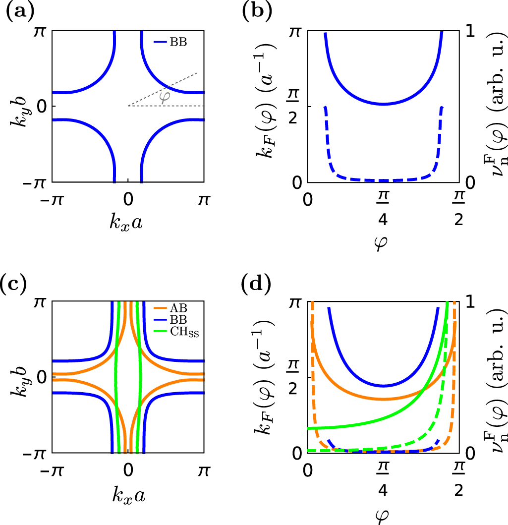
The used tight binding parameters are summarized in table 1. The calculated Fermi surface in the first Brillouin zone (BZ) is shown in figures 4(a) and (c) for Bi2212 and Y123. An analytic expression for the Fermi wave vector  is retrieved from the solution of
  where
where  is the polar representation of equation (6). The normal DOS is then given by

Figure 4. Normal state electrons: (a)and (c) Calculated Fermi surface in the first 2D BZ of Bi2212 (a) and Y123 (c). (b) and (d) Calculated Fermi wave vector  (solid line) and normal conducting DOS along the Fermi surface contour
  (dashed line) as function of polar angle in the first BZ quadrant (sketched in (a) for Bi2212 (b) and Y123 (d). Colors match the Fermi surface contours of the individual bands (AB, BB, CH
 ) from (a) and(c).
Download figure:
Standard image High-resolution imageTable 1. Tight binding parameters: Chemical potential µ and hopping parameters ti used in the dispersion relation for the Bi2212 and Y123 bands (equations (6) and (7)).
| Band | µ | t1 | t2 | t3 | t4 | t5 | |
|---|---|---|---|---|---|---|---|
| Bi2212 | |||||||
| BB | −0.1305 | −0.5951 | 0.1636 | −0.0519 | −0.1117 | 0.051 | |
| Y123 | |||||||
| BB | −0.38 | −1.1259 | 0.5540 | −0.1774 | 0.0701 | 0.1286 | |
| AB | −0.515 | −1.0939 | 0.5112 | −0.0776 | −0.1041 | 0.0674 | |
| ta | tb | ||||||
CH
| −0.2155 | −0.12 | −0.0035 | — | |||

where  is a parametrization of the path along the Fermi surface,
  is the Euclidean norm and
  . It is shown as a function of the polar angle ϕ in figures 4(b) and (d) for Bi2212 and Y123 respectively.
Appendix B: The numerical scaling factor η
To approximate η, we used the boundary condition

i.e. the total number of electronic states is conserved in the phase transition from the normal to the superconducting phase. The integral is bound by the band width. This procedure is depicted in figure 5(a).

Figure 5. Numerical scaling factor: (a) Determination of η through the boundary condition equation (9). (b) Variation of η leaves the general shape of the extracted bosonic spectrum unaffected except for the magnitude of its zero-energy peak.
Download figure:
Standard image High-resolution imageIn order to make sure that the introduction of the numerical scaling factor η has no poisoning effect on our extracted bosonic spectrum, the deconvolution of the Bi2212 spectrum by Gold's algorithm was performed for four different values of η. The results shown in figure 5(b) are comforting in the sense that the overall shape of the bosonic spectrum is unchanged. The only major difference lies in the magnitude of the zero-energy peak which is to be expected from a scalar multiplication, but since this peak is anyhow out of the bounds of physical contributions it does not harm the analysis.
Appendix C: LDOS inhomogeneity
As reported by Fischer et al Bi2212 tends to show a large inhomegeneity of its LDOS in the superconducting state [66]. This can be confirmed in our experiment by direct comparison of the conductance inhomogeneity measured on Bi2212 and Y123, shown in figure 6. The heat maps of the conductance variation

show that it is about three times higher on the Bi2212 surface than on the Y123 surface. As a consequence, a position averaged spectrum over a  area can preserve detailed gap features better for Y123 than for Bi2212. Especially the dip-hump (dip marked by blue, hump marked by red arrows in figure 6 feature is still clearly visible in the position averaged spectrum of Y123 at
  but is invisible in Bi2212. The preservation of this feature in the spectrum is crucial for our ITS analysis. Therefore, in the case of Bi2212, an average spectrum at one specific location, at which the dip-hump spectral feature was clearly visible, was chosen for this study. For Y123, the position averaged spectrum was chosen

Figure 6. LDOS inhomogeneity: Position averaged bias spectra on a  area at
  for Bi2212 (a) and Y123 (b). Heat maps in the inset show the variation of the differential conductance within the averaging area. The higher inhomogeneity of the Bi2212 surface is reflected in both the conductance variation map and the blurred position averaged spectrum. The characteristic dip and hump are marked by blue and red arrows.
Download figure:
Standard image High-resolution image