

Abstract
An analytical bond-order potential (BOP) of Fe–Bi has been constructed and has been validated to have a better performance than the Fe–Bi potentials already published in the literature. Molecular dynamics simulations based on this BOP has been then conducted to investigate the ground-state properties of Bi, structural stability of the Fe–Bi binary system, and the effect of Bi on mechanical properties of BCC Fe. It is found that the present BOP could accurately predict the ground-state A7 structure of Bi and its structural parameters, and that a uniform amorphous structure of Fe100−xBix could be formed when Bi is located in the composition range of 26 ⩽ x < 70. In addition, simulations also reveal that the addition of a very small percentage of Bi would cause a considerable decrease of tensile strength and critical strain of BCC Fe upon uniaxial tensile loading. The obtained results are in nice agreement with similar experimental observations in the literature.
Export citation and abstract BibTeX RIS
1. Introduction
Iron–bismuth (Fe–Bi) is an immiscible binary system with a positive heat of formation (+18 kJ mol−1) [1] and has raised a lot of research interests during the past decades. On the one hand, Fe–Bi nanoparticles and multilayers possess unique magnetic properties and have been potentially used in some industrial and biomedical fields such as computer tomography and magnetic resonance imaging [2–7]. Interestingly, metastable rhombohedral and body-centered-cubic (BCC) solid solutions as well as amorphous structures of Fe–Bi have been experimentally fabricated by ion beam mixing [8], magnetron sputtering [3, 4, 7], electron-beam evaporation [2, 9, 10], mechanical alloying [11], etc. On the other hand, the interaction between Fe and Bi seems important in nuclear power systems, as Bi and its alloys are a first-choice candidate of spallation target and coolant, which induce the corrosion and liquid metal embrittlement (LME) of stainless steels and affect the safety operation of the nuclear reactors [12–14].
It is well known that molecular dynamics (MD) simulation based on a realistic n-body potential is a capable way to predict various structures and properties of a binary system. In this respect, two Fe–Bi potentials have been already constructed within the framework of Lennard-Jones (LJ) and have been used to study the corrosion behavior of the Fe–Bi system [15, 16]. Moreover, a Bi–Bi potential has been derived under the formalism of embedded atom model (EAM) to simulate various properties of liquid Bi [17, 18]. However, we will show later that the above three potentials are failed to describe the ground-state rhombohedral structure (A7, space group No. 166, R
 m) of Bi [15–18] and are unable to predict the structural stability of metastable phases formed in the immiscible Fe–Bi system [15, 16].
Bond-order-potential (BOP) has been well regarded as a high-fidelity n-body potential based on molecular orbital theory and quantum mechanical tight binding models [19, 20]. As an angular dependent potential, BOP is especially appropriate for strong covalent-bonding materials such as Si, C, GaAs [21–24] and is also suitable for transition metals and alloys [19, 20, 25]. To our knowledge, however, there is not any BOP potential of Bi published so far in the literature. Therefore, a new n-body Fe–Bi potential is first constructed in the present study under the formalism of BOP [19, 20, 26–29]. Based on this Fe–Bi potential, MD simulations are performed to reveal the ground-state properties of the A7 structure of Bi, the structural stability of metastable phases of Fe–Bi, and the effects of Bi on mechanical properties of BCC Fe. It will be shown that the newly constructed Fe–Bi potential could correctly predict structural parameters and various properties of the ground-state A7 structure of Bi. The derived results from the present Fe–Bi potential simulations will be also discussed and compared with similar observations from the other potentials, experiments, and thermodynamical models in the literature [1, 15–18].
2. Construction of Fe–Bi bond-order potential
As related before, two LJ potentials and an EAM potential have been constructed for Bi and Fe–Bi [15–18], while it will be shown later that they are unstable to reproduce the ground-state rhombohedral structure (A7, space group No. 166, R
 m) of Bi as well as structural stability of Fe–Bi. In the present study, the Bi–Bi, Fe–Fe, and Fe–Bi potentials are therefore constructed based on the framework of BOP by Pettifor et al [26–29], and are compared extensively with the Fe–Bi potentials already in the literature.
According to the BOP formalism, the bond energy is the product of the bond-order and bond integral, and the total energy of a whole system with N atoms is expressed as [20]:
where rij is the distance between atoms i and j, ∅ij , βσ,ij , and βπ,ij are three pairwise functions, Θσ,ij and Θπ,ij are two variables which describe local circumstances around atoms i and j, and the list j = i1, i2, ..., iN represents neighbors of atom i. The first term of the right-hand side of equation (1) represent the overlap repulsion between a pair of ion cores [30]. βσ,ij and βπ,ij are σ and π bond integrals, respectively, while Θσ,ij and Θπ,ij are σ and π bond orders, respectively. The three pairwise funcitons have similar forms as:


where ∅0,ij
, βσ,0,ij
, βπ,0,ij
, mij
, and nij
are five pair-dependent parameters needed to be fitted. ∅0,ij
, βσ,0,ij
, βπ,0,ij
are three prefactors of repulsive energy, σ bond integral, and π bond integral, receptively.  is a Goodwin–Skinner–Pettifor (GSP) radial function written as [21]:

in which r0,ij
, rc,ij
, and nc,ij
are three pair-dependent parameters, and r0,ij
and rc,ij
are GSP reference radius and GSP characteristic radius, respectively.  is a cutoff function defined as:

where r1,ij
and rcut,ij
are two pair-dependent parameters to represent cutoff start radius and cutoff radius, respectively, and γij
and αij
can be obtained from ![${\gamma }_{ij}=\frac{\mathrm{ln}\left[\mathrm{ln}\left(0.99\right)/\mathrm{ln}\left(0.01\right)\right]}{\mathrm{ln}\left(\frac{{r}_{1,ij}}{{r}_{\mathrm{c}\mathrm{u}\mathrm{t},ij}}\right)}$](https://content.cld.iop.org/journals/0953-8984/34/2/025901/revision4/cmac2e8eieqn5.gif) and
and  .
.
The variable, Θσ,ij , is defined as
where  is the two-level σ bond order for the BOP approximation with a half-full valence shell,
  and
and  are local variables arising from the 2-hops, and
  is a local variable arising from the three-member ring hops [31]. ζ2 and ζ1, ζ3, ζ4 in the following equations (10) and (15) are global parameters, fσ,ij
and kσ,ij
are two pair-dependent parameters to be fitted.
is a local variable arising from the three-member ring hops [31]. ζ2 and ζ1, ζ3, ζ4 in the following equations (10) and (15) are global parameters, fσ,ij
and kσ,ij
are two pair-dependent parameters to be fitted.  is a function with continuous derivatives, and is expressed as the Ward's solution [31]:

where


The variable  in equations (7) and (8) is expressed as:
where cσ,ij
is a pair-dependent parameter. The variable  in equations (7) and (10) has the following form:

where θjik is the bond angle of atoms j–i–k, and gσ,jik (θjik ) is the angular function using the Ward's quadratic spline formula [20] as

where

in which g0,jik
, bσ,jik
and uσ,jik
are three three-body-dependent (jik) parameters to be fitted. It should be noted that the variable  in equations (7) and (10) is similar to
  with the bond angle of atoms i–j–k.
The term  in equation (7) is calculated as:
where k, j = n means that atoms k and j are neighbors.
The variable Θπ,ij in equation (1) is expressed as
where aπ,ij and cπ,ij are two pair-dependent parameters.
The term  is calculated as:
where pπ,i is an element-dependent parameter.
The term  in equation (15) can be written as:
with  and
and  .
.
In the above analytical functions of BOP, there are altogether four global parameters, seventeen parameters for single element Fe or Bi, and nineteen parameters for the Fe–Bi binary system needed to be determined. The following parameters can be determined according to the principles adopted by Ward et al [20] before the fitting process: the global parameters (ζ1, ζ2, ζ3, ζ4) and the three-body-dependent parameters g0,jik for Fe, Bi and Fe–Bi are set as the same values by Ward et al [20] and are shown in tables 1 and 3; the pair-dependent parameters (r0, rc , r1, rcut) for Fe, Bi and Fe–Bi are displayed in table 2; other selected parameters in table 2 are aπ = cπ = kσ = pπ = βπ = 0 and fσ = 0.5 for Fe, and aπ = cπ = 1 for Bi and Fe–Bi.
Table 1. Global and element-dependent BOP parameters for Bi and Fe.
| ζ1 | ζ2 | ζ3 | ζ4 | pπ,Bi | pπ,Fe |
|---|---|---|---|---|---|
| 0.000 01 | 0.000 01 | 0.001 | 0.000 01 | 0.477 904 | 0 |
Table 2. Pair-dependent BOP parameters for Bi, Fe, and Fe–Bi.
| Bi–Bi | Fe–Fe | Fe–Bi | |
|---|---|---|---|
| r0 (Å) | 3.1800 | 2.2452 | 2.7700 |
| rc (Å) | 3.1800 | 2.2452 | 2.7700 |
| r1 (Å) | 3.8200 | 2.7232 | 3.3800 |
| rcut (Å) | 4.3000 | 3.6492 | 3.9500 |
| nc | 3.497 238 | 3.289 429 | 4.441 948 |
| m | 1.994 330 | 1.046 363 | 1.211 758 |
| n | 1.107 474 | 0.461 114 | 0.622 392 |
| φ0 (eV) | 1.137 997 | 1.289 055 | 0.952 986 |
| βσ,0 (eV) | 0.468 553 | 1.306 371 | 1.272 759 |
| βπ,0 (eV) | 0.733 087 | 0 | 0.620 172 |
| cσ | 0.631 549 | 0.189 093 | 1.269 255 |
| fσ | 0.470 068 | 0.5 | 0.225 232 |
| kσ | 0.633 972 | 0 | 3.904 155 |
| cπ | 1 | 0 | 1 |
| aπ | 1 | 0 | 1 |
The remaining parameters should be obtained from a two-step fitting method as follows [20]. Based on equations (1)–(4), the bond energy (Eb,ij ) between atoms i and j can be expressed as:
At the equilibrium position, the first derivative ( ) of Eb,ij
equals zero and
) of Eb,ij
equals zero and

Substituting equation (19) in equation (18), the bond energy at the equilibrium position can be written as a function of equilibrium bond length:

Similarly, the second derivative ( ) of Eb,ij
could be derived as follows:
) of Eb,ij
could be derived as follows:

The atomic volume (Vij ), cohesive energy (Ec,ij ), and bulk modulus (Bij ) of a given structure can be then calculated through the following forms: [20]
where F is a structural volume factor, and Z is the atomic coordination.
For the first-step fitting, equations (20) and (22) are used to determine the pairwise GSP parameters (∅0, m, n, and nc ) through the fitting of Ec and B of each selected structure at the equilibrium volume from experiments or first principles calculations. Specifically, the structures of A7, BCC, FCC, HCP, and SC (simple cubic) are selected for Bi, the BCC, FCC, HCP, and SC structures are chosen for Fe, and the B1, B2, B3, B4, and C3 structures for Fe–Bi.
The second step of fitting is to obtain the remaining parameters (βσ,0, βπ,0, cσ , fσ , kσ , bσ , uσ ), i.e., the derived parameters (∅0, m, n, and nc ) in the first step are substituted into the right-hand side of equation (19) and treated as new reference values for the left-hand side of equation (19) during the fitting process. In addition, equations (18) and (22) are also used in the second step fitting, and the input data for equations (18) and (22) are the Ec values of the following structures from experiments or first principles calculations: A7 and BCC for Bi, BCC for Fe, and B1 and B2 for Fe–Bi.
It should be noted that the present first-principles calculations are performed through the Vienna ab initio simulation package (VASP) software [32]. The interaction between ion and valence electrons is described by the projector-augmented wave method [33, 34], and the exchange and correlation effect is expressed by the generalized gradient approximation [35–37]. The plane-wave cutoff energy is 500 eV for all the calculations. In addition, the temperature-smearing method of Methfessel–Paxton [38] and the tetrahedron method with Blöchl corrections [39] are performed for relaxation and static calculations during k space integration, respectively. The unit cells of A7, BCC, FCC, HCP, SC, B1, B2, B3, B4, and C3 structures contain 6, 2, 8, 2, 1, 8, 2, 8, 4, and 6 atoms, respectively, and their k-points are 15 × 15 × 7, 11 × 11 × 11, 11 × 11 × 5, 11 × 11 × 7, 11 × 11 × 11, 11 × 11 × 11, 11 × 11 × 11, 11 × 11 × 11, 11 × 11 × 7, and 11 × 11 × 11, respectively.
During the process of fitting, the properties of Bi with the A7 structure as well Fe with BCC and FCC structures have the higher weights than others. After a series of fitting, tables 1–3 summarize the optimized parameters of Bi, Fe, and Fe–Bi, and table 4 lists the obtained a, c, Ec, and B values of Bi, Fe, and FeBi with the selected structures from the present BOP, first principles calculations, and experiments [40–45]. It should be mentioned that the values of cohesive energy Ec from first principles calculations were shifted to experimental values according to the calculated energies differences for the sake of comparation. One can observe from table 4 that the constructed BOP has a generally nice performance in reproducing the Ec, and B values of Bi, Fe, and FeBi from experiments [40–45] and first principles calculation. The validation of the constructed Fe–Bi potential will be shown later in section 4.
Table 3. Three-body-dependent BOP parameters for Bi, Fe, and Fe–Bi.
| BiBiBi | FeFeFe | BiBiFe | BiFeBi | BiFeFe | FeBiFe | |
|---|---|---|---|---|---|---|
| g0,jik | 1 | 1 | 1 | 1 | 1 | 1 |
| bσ,jik | 0.488 041 | 0.920 095 | 0.862 671 | 0.557 518 | 0.698 533 | 0.830 309 |
| uσ,jik | −0.114 961 | −0.074 563 | −0.121 116 | −0.069 474 | −0.189 584 | −0.179 300 |
Table 4. Lattice parameters (a, c), cohesive energies (Ec), and bulk moduli (B) of Bi, Fe and FeBi with several selected structures from the present potential (BOP), first principles calculations (VASP), and experiments [40–45].
| Phase | Structure | a, c (Å) | Ec (eV/atom) | B0 (GPa) | ||||||
|---|---|---|---|---|---|---|---|---|---|---|
| BOP | VASP | Exp. | BOP | VASP | Exp. | BOP | VASP | Exp. | ||
| Bi | A7 | 4.563 | 4.540 | 4.546 [41] | −2.1803 | −2.180 | −2.18 [42] | 55 | 35 | 31 [40] |
| 11.827 | 11.577 | 11.865 [41] | ||||||||
| SC | 3.260 | 3.219 | −2.1798 | −2.144 | 58 | 50 | ||||
| FCC | 4.988 | 4.949 | −1.8631 | −2.059 | 87 | 54 | ||||
| BCC | 3.960 | 3.912 | −1.9328 | −2.085 | 88 | 54 | ||||
| HCP | 3.520 | 3.547 | −1.8613 | −2.083 | 87 | 52 | ||||
| 5.780 | 5.792 | |||||||||
| Fe | BCC | 2.866 | 2.832 | 2.866 [45] | −4.2832 | −4.280 | −4.28 [42] | 163 | 185 | 169 [43] |
| FCC | 3.680 | 3.539 | 3.640 [45] | −4.2750 | −4.179 | 133 | 172 | 133 [44] | ||
| SC | 2.160 | 2.373 | −3.4324 | −3.515 | 120 | 103 | ||||
| HCP | 2.602 | 2.430 | −4.2762 | −4.189 | 135 | 290 | ||||
| 4.249 | 3.968 | |||||||||
| FeBi | B1 | 5.737 | 5.594 | −2.4868 | −2.562 | 65 | 62 | |||
| B2 | 3.431 | 3.415 | −2.4813 | −2.640 | 76 | 75 | ||||
| B3 | 6.151 | 6.161 | −2.3085 | −2.299 | 38 | 36 | ||||
| B4 | 4.351 | 4.353 | −2.3085 | −2.297 | 34 | 38 | ||||
| 7.106 | 7.108 | |||||||||
| Fe2Bi | C3 | 6.100 | 5.982 | −1.6124 | −1.757 | 12 | 32 | |||
| FeBi2 | C3 | 6.019 | 5.636 | −2.0451 | −2.156 | 32 | 48 | |||
3. Simulation methods
Based on the newly constructed BOP of Fe–Bi, the present MD simulations are performed by means of the well-known software of large-scale atomic/molecular massively parallel simulator package [46]. Accordingly, the Fe100−x
Bix
solid solutions are constructed within the entire composition range of 0 ⩽ x ⩽ 100 with an interval of x = 2. Two structures of BCC and A7 are selected at each composition of Fe100−x
Bix
, and the unit cells of 68 × 68 × 68 Å3 (16 000 atoms) and 81.6 × 86.4 × 82.7 Å3 (16 632 atoms) are chosen for BCC and A7 structures, respectively. The x, y, and z directions of the unit cell are set along [100], [010], and [001] for the BCC structure, respectively, while [ ], [
], [ ], and [0001] for the A7 structure, respectively. For each composition of Fe100−x
Bix
, the unit cell is formed by randomly substituting Fe (or Bi) atoms by Bi (or Fe) atoms. Periodic boundary conditions are added at three directions of the unit cell, and each solid solution is relaxed at 0.1 K under the isothermal-isobaric (NPT) ensemble for 50 ps and optimized through the conjugate gradient method. It should be noted that for BCC or A7 structure at each composition of Fe100−x
Bix
, five samples are considered for random substitutions, and the data shown in the following tables and figures are average values. The relative errors of the calculated lattice parameters, cohesive energies, elastic constants and moduli, surface energies, heat capacities, and heat of formation are within 0.001%, 10−6 %, 2%, 1%, 1%, and 5%, respectively.
], and [0001] for the A7 structure, respectively. For each composition of Fe100−x
Bix
, the unit cell is formed by randomly substituting Fe (or Bi) atoms by Bi (or Fe) atoms. Periodic boundary conditions are added at three directions of the unit cell, and each solid solution is relaxed at 0.1 K under the isothermal-isobaric (NPT) ensemble for 50 ps and optimized through the conjugate gradient method. It should be noted that for BCC or A7 structure at each composition of Fe100−x
Bix
, five samples are considered for random substitutions, and the data shown in the following tables and figures are average values. The relative errors of the calculated lattice parameters, cohesive energies, elastic constants and moduli, surface energies, heat capacities, and heat of formation are within 0.001%, 10−6 %, 2%, 1%, 1%, and 5%, respectively.
4. Result and disscusion
It is of importance to validate the newly constructed BOP of Bi–Bi, Fe–Fe, and Fe–Bi. After a series of MD simulations, it will show that the present BOP of Fe–Bi could correctly predict the ground state A7 structure of Bi, reveal the structural stability of Fe–Bi phases, and find out the effects of Bi on mechanical properties of BCC Fe. The simulated results from the present potential are in good agreement with experimental data in the literature, and the present BOP of Fe–Bi has a better performance to reflect the intrinsic properties of the binary Fe–Bi system than the two LJ potentials and an EAM potential have been constructed for Bi and Fe–Bi [15–18].
4.1. Ground-state structure and properties of Bi
It is well known that the ground-state structure of Bi is a rhombohedral structure of A7 (space group No. 166, R
 m, Pearson symbol hR2) with a special rhombohedral angle (θrh) of 57.23° [41]. This structure can be also recognized as a hexagonal structure with a unique internal parameter of u = 0.2340 as a result of its layered atomic arrangement [47]. The A7 structure of Bi and its equivalent hexagonal structure are shown vividly in figure 1. Such a special angle of θrh and an internal parameter of u make it difficult to accurately reproduce the ground-state structure of Bi by an n-body potential. Probably due to this difficulty, the A7 structure has been simply disregarded by the EAM and two LJ potentials of Bi in the literature and the BCC structure of Bi is used for the fitting instead [15–18]. In the present study, BOP has been intentionally selected to construct the potential of Bi due to its suitability for directional bonding, and it is therefore of importance to see whether or not the constructed BOP of Bi could reflect the ground-state structure and properties of Bi. The properties from the EAM and two LJ potentials of Bi already in the literature are also included for the sake of comparison.

Figure 1. Rhombohedral (A7) and hexagonal unit cell of Bi bulk. The brown and green atoms distinguish the atoms in the two layers of each bilayer.
Download figure:
Standard image High-resolution imageConsequently, figure 2 shows the comparison of energy curves of Bi with the structures of A7, BCC, FCC, HCP, and SC obtained from the potentials of the present BOP, EAM [17, 18], as well as LJ of Maulana [16] and Liu [15]. It can be seen clearly from figure 2(a) that the A7 structure is predicted by the present BOP to possess the lowest energy among the selected structures, and is therefore regarded as the ground-state structure of Bi, which agrees well with the ground-state A7 structure of Bi from experimental observations in the literature [41, 42]. On the contrary, the energy curves in figure 2 from the EAM and LJ potentials of Bi reveal that the HCP or FCC structure has the lowest energy, which seems contradictory to the ground-state A7 structure by experiments [41, 42].
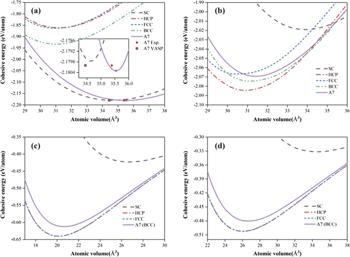
Figure 2. Energy curves of Bi with the structures of A7, BCC, FCC, HCP, and SC (simple cubic) obtained from the potentials of (a) the present BOP, (b) EAM [17, 18], as well as LJ of (c) Maulana [16] and (d) Liu [15]. The data point of the A7 structure of Bi from the present first principles calculation (VASP) is also included in (a).
Download figure:
Standard image High-resolution imageTable 5 summarizes the derived cohesive energy (Ec), lattice parameters (a, arh and c/a), internal parameter (u), and rhombohedral angle (θrh) of the A7 structure of Bi obtained from the present BOP, experiments [41, 42], EAM potentials [17, 18], and LJ potentials of Maulana [16] and Liu [15]. One could discern from this table that the present BOP could accurately predict the structural parameters of the ground-state A7 structure of Bi. For instance, the arh, u, and θrh of A7 from the present study are 4.741 Å, 0.2369, and 57.53°, respectively, which match well with the corresponding experimental values of 4.746 Å, 0.2340, and 57.23°. Unfortunately, the EAM and LJ potentials of Bi [15–18] could not correctly reproduce the cohesive energy and structural parameters of the A7 structure due to the big differences of the calculated and experimental values shown in table 5.
Table 5. Cohesive energy (Ec), lattice parameters (a, arh and c/a), internal parameter (u), and rhombohedral angle (θrh) of the A7 structure of Bi obtained from the present potential (BOP), experiments [41, 42], EAM potentials [17, 18], and the LJ potentials of Maulana [16] and Liu [15].
| Ec (eV/atom) | a (Å) | arh (Å) | u | c/a | θrh (°) | |
|---|---|---|---|---|---|---|
| BOP | −2.1803 | 4.563 | 4.741 | 0.2369 | 2.592 | 57.53 |
| Exp. [41, 42] | −2.18 | 4.546 | 4.746 | 0.2340 | 2.610 | 57.23 |
| EAM [17, 18] | −2.0693 | 5.618 | 4.138 | 0.2491 | 1.229 | 86.79 |
| LJ [16] | −0.6123 | 4.889 | 3.457 | 0.2500 | 1.225 | 90 |
| LJ [15] | −0.4803 | 5.326 | 3.767 | 0.2500 | 1.225 | 90 |
In addition, the elastic constants of the A7 structure of Bi are calculated through the relationship of energy and strain [48], and the obtained results are displayed in table 6. The C11, C14, and C44 values of the A7 structure from the present BOP are in accordance with experimental measurements [40], while the present potential overestimates the C12, C13, and C33 values. One could also observe that the elastic constants from the EAM potential [17, 18] are much bigger than the experimental values [40], and that the present BOP has a much nicer agreement with experiments than the EAM potential. It should be pointed out that the A7 structure of Bi from the two LJ potentials [15, 16] becomes mechanically unstable and its elastic constants are thus unavailable.
Table 6. Elastic constants Cij (GPa) and bulk moduli B (GPa) of A7 structure of Bi as well as BCC and FCC structures of Fe from the present potential (BOP), the present first principles calculation (VASP), experiments [40, 43, 44], EAM potentials of Bi [17, 18] and Fe [51], and the LJ potentials of Maulana [16] and Liu [15].
| Phase | Structure | Cij | BOP | VASP | Exp. [40, 43, 44] | EAM [17, 18, 51] | LJ [16] | LJ [15] |
|---|---|---|---|---|---|---|---|---|
| Bi | A7 | C11 | 66 | 84 | 69.3 | 106 | Unstable | Unstable |
| C12 | 47 | 24 | 24.5 | 53 | Unstable | Unstable | ||
| C13 | 52 | 35 | 25.4 | 58 | Unstable | Unstable | ||
| C14 | 4 | 21 | 8.4 | −28 | Unstable | Unstable | ||
| C33 | 73 | 58 | 40.4 | 168 | Unstable | Unstable | ||
| C44 | 16 | 41 | 13.5 | 195 | Unstable | Unstable | ||
| Fe | BCC | C11 | 223 | 258 | 226 | 229 | 1187 | 679 |
| C12 | 133 | 149 | 140 | 135 | 499 | 387 | ||
| C44 | 100 | 96 | 116 | 116 | 499 | 146 | ||
| Fe | FCC | C11 | 196 | 253 | 154 | 107 | 876 | 679 |
| C12 | 101 | 131 | 122 | 98 | 499 | 387 | ||
| C44 | 98 | 106 | 77 | 80 | 499 | 387 |
The surface energy and heat capacity of the A7 structure of Bi are also calculated by MD simulation with the present BOP, and the results are shown in table 7. The corresponding experimental value [49] as well as available calculated data from first principles calculation [50] and EAM potential [17, 18] are also listed in table 7 for comparison. The present surface energy (0.17 J m−2) of the (111) surface of Bi matches well with the corresponding value of 0.16 J m−2 from first principles calculations [50], whereas such a value of 0.44 J m−2 from the EAM potential [17, 18] seems much bigger. Moreover, the volumetric heat capacity of the A7 structure of Bi at 283 K from the present BOP is compatible with the corresponding values from experiments [49] and the EAM potential [17, 18].
Table 7. Surface energy Es (J m−2) and heat capacity Cv (J·mol−1·K−1) at 283 K of A7 Bi and BCC Fe from the present potential (BOP), experiments [49, 52, 53], first principles calculation [50, 54], EAM potentials of Bi and Fe [17, 18, 51], and the LJ potentials of Maulana [16] and Liu [15]. The experimental Es of Fe is surface energy of polycrystalline sample.
| Bi | Fe | |||||
|---|---|---|---|---|---|---|
| Es (111) | Cv | Es (100) | Es (110) | Es (111) | Cv | |
| BOP | 0.17 | 28.5 | 2.06 | 1.89 | 2.34 | 25.3 |
| Exp. [49, 52, 53] | — | 25.9 | 2.36 | 25.6 | ||
| Cal. [50, 54] | 0.16 | — | 2.29 | 2.27 | 2.52 | — |
| EAM [17, 18, 51] | 0.44 | 28.2 | 1.70 | 1.43 | 1.94 | 25.1 |
| LJ [16] | — | — | 5.89 | 5.65 | 6.28 | 24.2 |
| LJ [15] | — | — | 4.68 | 4.48 | 4.98 | 24.3 |
From the above simulated results, one can see clearly that the constructed BOP of Bi is not only able to successfully predict the ground-state A7 structure of Bi and its structural parameters, but also capable of reproducing the elastic constants, surface energy, and heat capacity of the A7 structure of Bi. These nice agreements with experiments validate the relevance of the present BOP of Bi. The EAM and LJ potentials of Bi already in the literature [15–18], however, are unable to reflect the ground-state A7 structure of Bi and its structural parameters. It should be noted that the present BOP potential of Bi has been constructed, and this BOP potential of Bi has been therefore used to derive the Fe–Bi cross potential, the validation of which will be presented in the following sections.
Additionally, it is of interest to see the performance of the BOP of Fe. After a series of calculations, table 6 lists the obtained elastic constants (C11, C12, C44) of Fe with the BCC and FCC structures, and table 7 shows the calculated surface energies (Es), and heat capacity (Cv ) of BCC Fe. One can discern clearly from these two tables that the C11, C12, C44, Es, and Cv values of Fe from the present BOP are compatible with corresponding experimental and calculated data in the literature [43, 44], suggesting that the constructed BOP of Fe is realistic to reflect the intrinsic feature of Fe. As shown also in table 7, the EAM potential [51] has a similar performance to reproduce the elastic constants and heat capacity of Fe as the present BOP, while underestimates the surface energy of Fe. On the other hand, the two LJ potentials [15, 16] considerably overestimate the elastic constants and surface energy of Fe.
4.2. Structural stability of Fe–Bi phases
As related before, Fe–Bi is an immiscible binary system with a positive heat of formation (+18 kJ mol−1) [1], while metastable Fe–Bi phases with the BCC and A7 structures have been fabricated by ion beam mixing [8], magnetron sputtering [3, 4, 8], electron-beam evaporation [2, 9, 10], and mechanical alloying [11], etc. Interestingly, amorphous Fe–Bi phases have been also discovered experimentally when the Bi composition is in the range of 40–60 at.% and 10–30 at.% [8–10]. As to theoretical studies about the metastable Fe–Bi phases, however, there is not any investigation so far in the literature. Based on the newly constructed BOP of Fe–Bi, the present study is therefore dedicated to find out the structural stability of the binary Fe–Bi system.
Accordingly, the unit cells of Fe100−x Bix solid solutions with the BCC and A7 structures are constructed, respectively, within the entire composition range at an x interval of 2. Each Fe100−x Bix solid solution is obtained through a random substitution of Fe (or Bi) atoms with Bi (or Fe). After relaxation, it is found that the Fe100−x Bix solid solutions could keep the BCC or A7 structure when x is within a certain range. On the other hand, the BCC or A7 structure of Fe100−x Bix solid solutions would become unstable, and will completely or partially transform to amorphous structure when x exceeds a specific composition. The revealed composition ranges of the BCC, A7, and amorphous structures of Fe100−x Bix will be described in the following paragraphs.
The heat of formation (ΔHf) of each Fe100−x Bix phase with the BCC, A7, or amorphous structure is calculated by the following form:

where  represents the total energy of each Fe100−x
Bix
phase, EBi and EFe are totals energies of the ground-state A7 and BCC structures for Bi and Fe, respectively. It should be mentioned that the term of the product of pressure and volume is not included in equation (23) due to the zero pressure maintained during the present MD simulations. After the calculations, figure 3 shows the heats of formation of the Fe100−x
Bix
phases obtained from the present study, the LJ potentials of Maulana [16] and Liu [15], as well as the thermodynamic model of Miedema et al [1]. In addition, figures 4 and 5 display, as typical examples, the atomic configurations and radial distribution functions of several Fe100−x
Bix
phases, respectively, and figure 6 shows the partial radial distribution functions of Fe–Fe, Fe–Bi, and Bi–Bi in the amorphous structure of Fe50Bi50.
represents the total energy of each Fe100−x
Bix
phase, EBi and EFe are totals energies of the ground-state A7 and BCC structures for Bi and Fe, respectively. It should be mentioned that the term of the product of pressure and volume is not included in equation (23) due to the zero pressure maintained during the present MD simulations. After the calculations, figure 3 shows the heats of formation of the Fe100−x
Bix
phases obtained from the present study, the LJ potentials of Maulana [16] and Liu [15], as well as the thermodynamic model of Miedema et al [1]. In addition, figures 4 and 5 display, as typical examples, the atomic configurations and radial distribution functions of several Fe100−x
Bix
phases, respectively, and figure 6 shows the partial radial distribution functions of Fe–Fe, Fe–Bi, and Bi–Bi in the amorphous structure of Fe50Bi50.
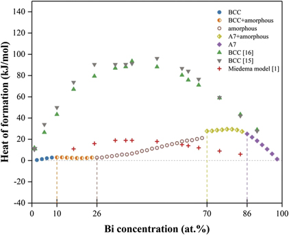
Figure 3. Heats of formation of Fe100−x Bix phases obtained from the present study, the LJ potentials of Maulana [16] and Liu [15], as well as the thermodynamic model of Miedema et al [1].
Download figure:
Standard image High-resolution image
Figure 4. Atomic configurations of (a) BCC + amorphous of Fe90Bi10, (b) amorphous of Fe50Bi50, (c) A7 + amorphous of Fe30Bi70, and (d) A7 of Fe14Bi86. The blue and brown balls represent Fe and Bi atoms, respectively. The x, y, and z directions are along [100], [010], [001] of the BCC structure, and along [ ], [
], [ ], [0001] of the A7 structure, respectively.
Download figure:
Standard image High-resolution image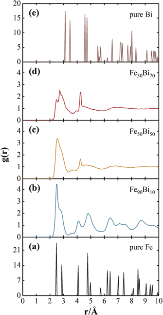
Figure 5. Radial distribution functions of (a) BCC Fe, (b) Fe90Bi10, (c) Fe50Bi50, (d) Fe30Bi70, and (e) A7 Bi.
Download figure:
Standard image High-resolution image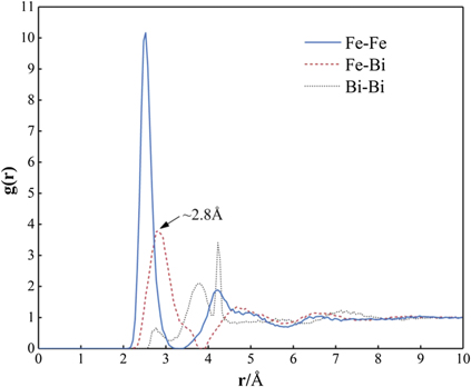
Figure 6. Partial radial distribution functions of Fe–Fe, Fe–Bi, and Bi–Bi in the amorphous structure of Fe50Bi50.
Download figure:
Standard image High-resolution imageSome features of structural stability of Fe100−x Bix phases could be discerned from figures 3–6. First of all, the heats of formation of the energetically favorable Fe100−x Bix phases obtained from the present study are compatible with those from the thermodynamic model of Miedema et al [1], although some apparent discrepancy exists between the present and thermodynamic values within some composition ranges shown in figure 3. This discrepancy would be probably due to the fact that crystal structure was not considered during thermodynamic calculations [1]. On the other hand, the two LJ potentials of Fe–Bi [15, 16] significantly overestimate the heats of formation of BCC Fe100−x Bix phases, and could not simulate the A7 structure of Fe100−x Bix due to its instability.
Secondly, the Fe100−x Bix phases could keep the BCC and A7 structures when 0 ⩽ x < 10 and 86 ⩽ x ⩽ 100, respectively. By means of mechanical alloying, Grigorieva et al discovered that Fe97Bi3 has a single BCC structure [11], and the composition of Fe97Bi3 is just located within the predicted composition range (0 ⩽ x < 10) of BCC Fe100−x Bix phases. Moreover, Bi atoms are experimentally found to dissolve in the BCC lattice of Fe, and Fe atoms are discovered to substitute the Bi atoms in the A7 structure [3, 9], which are also in accordance with the above simulated results.
Thirdly, the BCC Fe100−x Bix phases become partially amorphous when 10 ⩽ x < 26, i.e., BCC + amorphous. As a typical example to vividly show the mixture of BCC and amorphous, one can see from figure 4(a) that some disordered regions called amorphous have been formed in the atomic configurations of Fe90Bi10, while its BCC structure can be still apparently discerned. In addition, the radial distribution functions of Fe90Bi10 displayed in figure 5(b) also have typical features of both BCC and amorphous structures, i.e., the original sharp peaks of BCC shown in figure 5(a) have been broadened or disappeared when the Bi composition reaches the critical point of 10 at.%.
Fourthly, on the Bi-rich side, partial amorphization (A7 + amorphous) of the A7 Fe100−x Bix phases could be also realized when the Bi composition is within the range of 70 ⩽ x < 86. Compared with the A7 structure of Fe14Bi86 in figure 4(d), the atomic configuration of Fe30Bi70 in figure 4(c) exhibits a largely disordered pattern, whereas the A7 structure could be observed to some extent. Such a mixture of A7 + amorphous of Fe30Bi70 could also be seen in terms of pair correlation function in figure 5(d). Interestingly, the partial amorphization (A7 + amorphous) of FeBi phases was indeed observed experimentally [2, 9], which is in nice agreement with the above simulated results from the present BOP of Fe–Bi.
Fifthly, a uniform amorphous structure of Fe100−x Bix could be formed when the composition of Bi is located in the range of 26 ⩽ x < 70. Figure 4(b), as a typical example, displays the atomic configurations of the obtained amorphous structure of Fe50Bi50. A completely disordered pattern has been formed in Fe50Bi50, and the BCC or A7 structure could no longer be discerned in figure 4(b). Moreover, figure 5(c) also shows the pair correlation function of Fe50Bi50, which has a typical feature of amorphous with only a short-range order.
It is of importance to compare the above simulation results regarding amorphous Fe100−x Bix with similar experimental observations in the literature. Chen et al discovered that the Fe100−x Bix phase becomes a uniform amorphous structure when Bi is in the range of 40–60 at.% and 45–60 at.% after ion-beam mixing [8] and electron beam codeposition [9], respectively. Such experimentally-observed composition ranges are just located within the above predicted range of 26 ⩽ x < 70 for amorphous structure of Fe100−x Bix , and it seems understandable that the present theoretical composition range of amorphous formation seems a little bigger. By means of experiments, Forester et al also identified the partial amorphization of Fe100−x Bix when 10 ⩽ x ⩽ 30 [10], which is in good agreement with the present predicted composition of 10 ⩽ x < 26 for the BCC + amorphous structure of Fe100−x Bix . Furthermore, the atomic distance of Fe–Bi in the amorphous structure of Fe50Bi50 is experimentally measured to be 2.8 Å [8], which matches well with the present simulated value of 2.8 Å shown in figure 6.
All the above points indicate that the present MD simulation based on the newly constructed BOP of Fe–Bi is able to reveal the structural stability of the binary Fe–Bi system in terms of metastable phase formation. The predicted BCC, BCC + amorphous, amorphous, A7 + amorphous, and A7 structures of Fe100−x Bix phases within the entire composition range agree well with similar experimental observations in the literature [2, 3, 8–11]. These nice agreements therefore provide a strong support for the validation of the newly constructed BOP of Fe–Bi. Nevertheless, it should be pointed out that the two LJ potentials [15, 16] are unable to reflect the structural stability of various Fe–Bi phases.
4.3. Effects of Bi on mechanical properties of BCC Fe
It is commonly believed that Bi and its alloys are promising candidates of spallation target and coolant with superior properties in nuclear power systems. The interaction between Fe and Bi, however, has been a challenging issue among scientists and engineers, as Bi and its alloys are found to corrode the structural materials, and bring about the so-called LME of ferrite/martensite stainless steels, the mechanism of which has been still controversial during the past decades [12–14]. In the present MD simulations, it is therefore of importance to find out the effect of Bi on elastic properties and stress–strain relationships of BCC Fe based on the newly constructed Fe–Bi potential.
After a series of calculations, figure 7 shows the obtained elastic constants (C11, C12, C44), elastic moduli (B, G, E), and G/B ratios of BCC Fe100−x Bix phases as a function of Bi composition. It should be noted that five compositions of Fe100−x Bix with an interval of x = 2 have been selected in figure 7 and the maximum composition of Bi is 8 at.%, as the stable range of the BCC structure of Fe100−x Bix is 0 ⩽ x < 10 as derived before. One can observe from figure 7 that the addition of Bi has an important effect to reduce the elastic constants and elastic moduli of BCC Fe, and such a decrease become more apparent with the increase of Bi composition. This effect of Bi would be probably ascribed to the much lower elastic constants of Bi than those of Fe as shown in table 6.
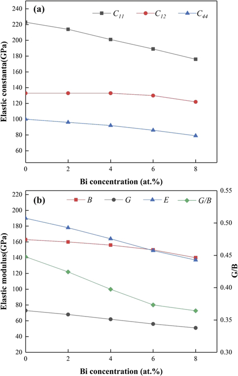
Figure 7. (a) Elastic constants (C11, C12, C44) and (b) elastic moduli (B, G, E), and G/B ratios of BCC Fe–Bi phases.
Download figure:
Standard image High-resolution imageThe G/B ratios of these five BCC Fe100−x Bix phases are also calculated and are displayed in figure 7. It should be pointed out that the G/B ratio has been universally regarded as a criterion to express the brittle/ductile behavior of a materials, i.e., a smaller G/B less than the critical value of 0.57 signifies a more ductile feature, and vice versa. Interestingly, the G/B ratios shown in figure 7 decrease with the increase of the Bi composition, suggesting that the addition of Bi could make it more ductile for BCC Fe, which is apparently contradictory to the experimental observation of the brittle behavior of BCC steels due to the effect of Bi [12–14]. Such a disagreement indicates that the G/B ratio in the elastic range should be unsuitable to describe the effect of Bi on the brittle/ductile behavior of BCC Fe, and that plastic deformation would probably occur during the experimental brittle process of the Fe–Bi system [12–14].
Furthermore, figure 8 displays, as typical examples, the stress–strain curves of BCC Fe100−x Bix phases with four Bi compositions (x = 0.0065, 0.1, 1, and 2) under a uniaxial tensile loading along the [111] direction. Each tensile loading is performed at 0.1 K with a constant engineering strain rate of 1 × 10⁹ s−1 and a timestep of 0.001 ps under the NPT ensemble. The corresponding stress–strain curve of BCC Fe is also included in figure 8 for the sake of comparison. It should be pointed out that the maximum Bi composition shown in figure 8 is 2 at.%, since the BCC structure of Fe100−x Bix is found to become unstable with an incorrect stress–strain curve under a uniaxial loading when x is bigger than 2.
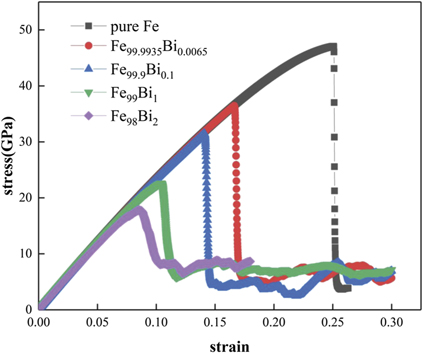
Figure 8. Stress–strain curves of BCC Fe100−x Bix phases when x = 0, 0.0065, 0.1, 1, and 2 under a uniaxial tensile loading along the [111] direction.
Download figure:
Standard image High-resolution imageOne can discern clearly from figure 8 that the stress–strain curve of BCC Fe100−x Bix phase when x = 0.0065 is apparently lower with a much smaller critical strain than that of pure BCC Fe, implying that a very small percentage (0.0065 at.%) of Bi could considerably reduce the tensile strength and ductility of BCC Fe. Moreover, both tensile strength and critical strain of BCC Fe100−x Bix phases decrease with the increase of the Bi composition. In other words, the addition of Bi would significantly increase the brittleness of BCC Fe, which is in good agreement with similar experimental observations in the literature [12–14]. Such an agreement would provide further evidence for the relevance of the newly constructed BOP of Fe–Bi.
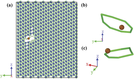
It is of interest to find out the fundamental reason why a very small percentage (0.0065 at.%) of Bi could considerably reduce the ductility of BCC Fe. Accordingly, figure 9 displays the atomic configuration and dislocation lines of the Fe1−x Bix phase (x = 0.0065 at.%) under uniaxial tensile loading along the [111] direction at the strain of 16.6%. As shown in figure 9, the addition of Bi has caused a considerable local distortion of the nearby Fe atoms and some dislocations lines of 1/2 ⟨111⟩ around the Bi atoms at the strain of 16.6%. Pure BCC Fe, however, only possesses a uniform deformation without any local distortion and dislocation lines during the uniaxial tensile loading (figures not shown). Such a local distortion and dislocations lines around the Bi atom would be probably attributed to the bigger atomic radius of Bi and the repulsive interaction between Bi and Fe, which could intrinsically bring about the much lower tensile strength and ductility of BCC Fe as shown in figure 8.
Figure 9. (a) Atomic configuration and (b) (c) dislocation lines of the BCC Fe100−x
Bix
phase (x = 0.0065 at.%) under uniaxial tensile loading along the [111] direction at the strain of 16.6%. The brown atom refers to the Bi atom and the figures are visualized with the software of OVITO. The x, y, and z directions are along [ ], [
], [ ], and [111], respectively.
Download figure:
Standard image High-resolution image
5. Conclusions
In summary, a new Fe–Bi potential of BOP has been constructed and has been proven to be more realistic than the LJ potentials of Fe–Bi already in the literature. Based on this BOP, the present MD simulation has been used to accurately reproduce the ground-state structure (A7) of Bi as well as its structural parameters and properties. Simulations also predict that the structures of BCC, BCC + amorphous, amorphous, A7 + amorphous, and A7 of Fe100−x Bix are energetically more favorable with less heat of formation when 0 ⩽ x < 10, 10 ⩽ x < 26, 26 ⩽ x < 70, 70 ⩽ x < 86, and 86 ⩽ x ⩽ 100, respectively. In addition, it is found that the addition of a very small percentage of Bi should have an important effect to significantly decrease the tensile strength of BCC Fe and considerably increase its brittleness. The obtained results are discussed and compared with experimental or theoretical results in the literature and the agreements between them are fairly nice.
Data availability statement
All data that support the findings of this study are included within the article (and any supplementary files).