
Abstract
In this topical review we catagorise all ambient pressure x-ray photoelectron spectroscopy publications that have appeared between the 1970s and the end of 2018 according to their scientific field. We find that catalysis, surface science and materials science are predominant, while, for example, electrocatalysis and thin film growth are emerging. All catalysis publications that we could identify are cited, and selected case stories with increasing complexity in terms of surface structure or chemical reaction are discussed. For thin film growth we discuss recent examples from chemical vapour deposition and atomic layer deposition. Finally, we also discuss current frontiers of ambient pressure x-ray photoelectron spectroscopy research, indicating some directions of future development of the field.
Export citation and abstract BibTeX RIS

Original content from this work may be used under the terms of the Creative Commons Attribution 4.0 licence. Any further distribution of this work must maintain attribution to the author(s) and the title of the work, journal citation and DOI.
1. Introduction
Since its original development by the group of Kai Siegbahn at Uppsala University in the mid-1960s, x-ray photoelectron spectroscopy (XPS) has become one of the most well-used and prolific experimental techniques in the fields of surface physics, surface chemistry and materials science (see e.g. Hüfner (2003)). The reasons for its usefulness are (i) its elemental specificity, which allows routine determination of the elemental composition of surfaces, (ii) its chemical specificity, which results from the presence of chemical shifts in the x-ray photoelectron (XP) spectra and which allows the elucidation of intricate details of the atomic- and molecular-scale structure of materials, (iii) its high surface sensitivity, which derives from the limited mean free path of relatively low-energy electrons in matter and (iv) its ease of use, especially for conducting and semiconducting materials. Particularly important for the success of XPS is the intimate relationship between the electronic and atomic-scale geometric structure of materials: XPS probes the electronic structure of a sample, and this knowledge allows to draw conclusions on the sample's geometric structure.
The original instruments for XPS, as well as for ultraviolet photoelectron spectroscopy (UPS), were all based on the use of laboratory sources, x-ray anodes and gas (especially helium) discharge lamps. Such laboratory-based setups continue to play an important role in the analysis of materials. Since the 1980s highly brilliant synchrotron radiation has become an enormously strong complement, which has made possible entirely new experiments on e.g. dilute samples, dynamics of electron processes, advanced depth profiling in materials, vibrational structure and other fine structure in XP and ultraviolet photoelectron (UP) spectra, and the rapid determination of band structure. For synchrotron-based experiments the tunability of the photon energy has made the distinction between UPS and XPS obsolete. Irrespective of photon energy, we will therefore refer to 'photoelectron spectroscopy' as 'XPS', although this is somewhat imprecise.
Conventionally, XPS makes use of vacuum environments at 10−5 mbar pressure or lower. The primary reason is the short mean free path of electrons in a gas phase. At kinetic energies up to some hundreds or around a thousand eV and at a pressure of 1 mbar it is on the order of millimetres, which is further reduced to the micrometre scale at atmospheric pressure. Additional reasons are the sensitivity of electron detectors to moisture and the requirement of keeping a solid surface clean for an extended period of time (on the order of hours), which can be achieved by keeping the solid sample in ultrahigh vacuum (UHV, 10−10 mbar and below).
The vacuum requirement of XPS—and other surface science techniques—turns out to be a limitation for the investigation of processes that require the presence of a phase interface. This is the case e.g. in heterogeneous catalysis, in corrosion and aerosol systems and in the study of solid state and liquid state chemistry. To overcome this limitation many surface science techniques have been developed further to enable the investigation of, in particular, the solid/gas interface. Examples of such methods are scanning tunnelling microscopy (Rasmussen et al 1998, Weeks et al 2000, Lægsgaard et al 2001, Kolmakov and Goodman 2003, Rößler et al 2005, Tao et al 2008, Herbschleb et al 2014, Onderwaater et al 2016), sum frequency generation (Rupprechter and Weilach 2008, Ozensoy and Vovk 2013), environmental transmission electron microscopy (Yoshida et al 2013, Xin et al 2013, Helveg et al 2014, Hansen and Wagner 2014, Crozier and Hansen 2015), environmental scanning electron microscopy (Danilatos and Robinson 1979, Danilatos 1981, Danilatos 1991, Thiel 2006) and operando x-ray absorption spectroscopy (Hävecker et al 1998, Knop-Gericke et al 2000, Lukashuk et al 2016).
XPS was adapted to higher pressure early on, already in the 1970s and 1980s (Siegbahn and Siegbahn 1973, Siegbahn 1985, Joyner and Roberts 1979, Ruppender et al 1990). The true breakthrough for ambient pressure x-ray photoelectron spectroscopy (APXPS) came, however, first with its introduction at synchrotron light sources and the combination of the necessary differential pumping stages between the sample environment and analyser with electrostatic focussing of the photoelectrons in the end of the 1990s and beginning of 2000s (Ogletree et al 2002). The new instruments made it possible to use APXPS to characterise chemical processes at a solid surface in an ambient atmosphere with a pressure of up to some ten mbar. As will be seen in section 2, the use of APXPS has grown rapidly since, and APXPS has found and continues to find applications in new scientific fields. Not least, the development of APXPS has contributed to a thorough revitalisation of the XPS field.
Many reviews have appeared on the topic of APXPS during the last decades. Reviews that limit themselves to a discussion of the APXPS technique and APXPS data can be found in e.g. Siegbahn (1985), Bukhtiyarov et al (2005), Bluhm et al (2007), Salmeron and Schlögl (2008), Knop-Gericke et al (2009), Ogletree et al (2009), Bluhm (2010), Starr et al (2013), Shavorskiy et al (2014a), Yoshida and Kondoh (2014), Mun et al (2014), Knudsen et al (2016), Kondoh et al (2016), Alayoglu et al (2016), Head and Schnadt (2016), Trotochaud et al (2017), Karslıoğlu and Bluhm (2017), Palomino et al (2017b), Olivieri et al (2017), Roy et al (2018), Weatherup (2018) and Arble et al (2018). Many more reviews exist that discuss particular scientific topics and which include APXPS data.
The present topical review serves two purposes: (a) we aim to update the APXPS publication statistics of Starr et al (2013) and to further refine them. (b) We would like to give our personal view on the frontiers of APXPS research, and some of them we will exemplify with results from our own research.
2. APXPS timeline and frontiers of APXPS research
Figure 1 shows an APXPS timeline for the time period from 1970 to 2018. The figure can be considered as an update of a similar figure in Starr et al (2013). It was, however, derived independently from literature searches for the terms ambient pressure x-ray photoelectron spectroscopy, near-ambient pressure x-ray photoelectron spectroscopy, APXPS, AP-XPS, NAPXPS, NAP-XPS, in situ XPS, high pressure x-ray photoelectron spectroscopy, HPXPS and HP-XPS. In addition, we added further APXPS publications that did not show up in the literature search, but that we were aware of. We note that some hard x-ray photoelectron spectroscopy (HAXPES) papers are included in our database, but we have made no systematic efforts to identify HAXPES publications that report data recorded under ambient or near-ambient conditions.
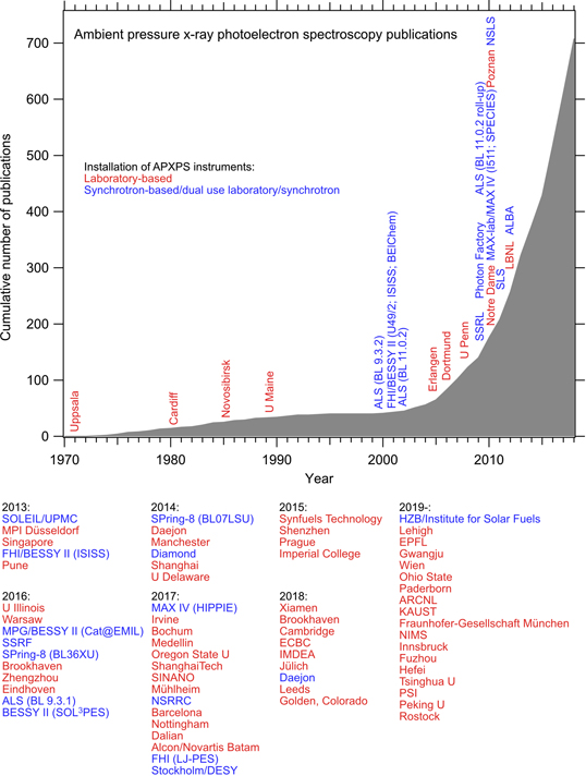
Figure 1. Updated APXPS timeline with data similar to those shown in Starr et al (2013). Shown are the cumulative number of publications and the dates of delivery/installation of new instruments, with synchrotron light-based instruments shown in blue and laboratory ones in red. Dates are given to the best of our knowledge; almost certainly further instruments exist, and not all instruments are in use anymore. At synchrotron radiation sources, some instruments have a history in terms of having subsequently been used at different beamlines. Where we are aware of such moves, we have indicated this by specification of the different beamlines.
Download figure:
Standard image High-resolution imageFor each publication the experimental conditions were verified, and only such papers were considered that report experiments at pressures of 10−3 mbar or more. Since not all APXPS publications contain one or more of the terms above, figure 1 needs to be considered as a conservative estimate. In this context we would like to encourage authors of APXPS papers to make sure that their publications use 'APXPS' or 'NAPXPS' as keywords. At the same time we would like to discourage the use of the term APPES for 'ambient pressure photoelectron spectroscopy', in spite of that it is sometimes more correct than 'APXPS'. The reason is that APPEs also stands for 'advanced pharmacy practice experiences', an established term in the US academic system and US scientific literature.
We note that the numbers reported in figure 1 are slightly lower than those in Starr et al (2013), especially in between 1990 and 2005 and in the very early years of APXPS, probably due to a different judgement of what to include and/or the difficulty in finding all relevant publications. This small difference notwithstanding, both the present timeline and that in Starr et al (2013) clearly show the impact of the APXPS activities that were started in the early 2000s at the Advanced Light Source in Berkeley and at BESSY-II in Berlin: from 2005 a strong rise in the number of publications is observed. The trend continues to-date, as is mirrored by the continued increase in the annual number of APXPS publications (2000: 1 paper, 2010: 36 papers, 2015: 54 papers, 2018: 95 papers).
In addition to the publication statistics figure 1 also contains the approximate installation dates of both the laboratory- and the synchrotron-based APXPS instruments that we are aware of. For the period between 1970 and 2012 the dates are indicated in the graph, while they are summarised below the graph for the time since 2013. The increasing number of APXPS instruments worldwide is another indicator for the continued growth of the field and the popularity of the method. It is interesting to observe that the period from 1999 to approximately 2012 is dominated by the installation of synchrotron-based instruments, while more recently laboratory-based instruments have taken over in terms of the number of installations. Arble et al (2018) provide an excellent overview of modern laboratory-based APXPS.
The timeline in figure 2 is based on the same set of data as figure 1, with the difference that now the publications have been categorised in terms of scientific area. The total number of publications is higher than in figure 1, since many APXPS papers report results from two and more scientific areas. This is especially true for the many review articles that have appeared during the past fifteen years. The inset shows the annual share of publications of different fields for the time span from 2000 to 2018.
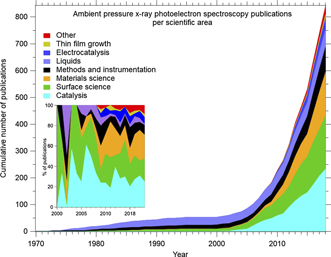
Figure 2. Categorisation of the APXPS papers published between 1970 and 2018 into scientific areas. The total number of papers is higher than that in figure 1 since many papers report data from than one scientific area. Review articles are included in the same way as publications that report original data. The inset shows the share of publications of respective field during each year between 2000 and 2018. The database underlying this data will eventually be made public at https://maxiv.lu.se/accelerators-beamlines/beamlines/hippie/apxps-training-materials/.
Download figure:
Standard image High-resolution imageThe categorisation is not necessarily unique; for example, many papers that report original catalysis data also report surface science or materials science data. Catalysis papers have only been included in the latter categories if the reported surface science or materials science data are substantial and have a clearly independent character of the catalysis data. Instead, they often have a supporting character, and then the publications have only been counted in the catalysis category. Conversely, both the surface science and materials science categories contain many publications with an outspoken catalysis background, but they do not report any data recorded under catalytic (generally gas mixture) conditions. Such papers have not been included in the catalysis category. Similarly, sometimes the delineation between the surface and materials science categories is somewhat arbitrary: publications have only been included in the surface science category if the samples have been well defined, as for example visible from the indication of Miller indices of the surface termination and/or the application of typical surface science sample cleaning methods such as sputtering and annealing. Otherwise, papers have been included in the materials science category. Publications that report XPS measurements on liquids have only been included if they have been recorded in the presence of an ambient vapour phase.
Figure 2 shows that catalysis, surface science and materials science are the predominant scientific areas in APXPS research. Instrument and method development have been and are important in the field. Experiments on liquids played a major role in the early days of APXPS and have gained increasing attention again during the last couple of years. Electrocatalysis has seen a strong increase during the past decade, and similarly, research on thin film growth has found its place in the APXPS research domain.
It is clear that the APXPS technique defines a vibrant and growing domain of materials research in a broad sense, encompassing fundamental physics and chemistry research as well as applied research on a large variety of different materials. The APXPS community is constantly seeking new challenges and problems that APXPS can be applied to. Therefore, there exist many different frontiers of APXPS research. Some of the frontiers that we identify are:
- (a)In catalysis research the investigation of more complex chemical reactions: as will be seen from the discussion in section 4, model reactions—such as the CO oxidation reaction—dominate APXPS research. Recently, investment into APXPS instruments has been considerable (cf figure 1), and the APXPS community will have to justify this investment by refining its ability to study real samples and catalytic reactions that are of primary relevance not only for surface scientist, but for a wider range of chemists in academia and industry. Below we will discuss some of the avenues that we have taken towards this goal.
- (b)The challenge of higher and even more realistic pressures than what present APXPS setups allow: even though pressures in the mbar and tens of mbar region are achieved routinely today, there remains the gap to truly realistic conditions, in particular in catalysis research. There are few industrial catalysis processes that are carried out at pressures below 1000 mbar. As demonstrated recently by Schlueter et al (2019) such pressures are in reach even for windowless APXPS setups, if the sample environment and gas dosing system are adapted accordingly and photon energies in the several keV-range are used. An alternative approach is to use ultrathin graphene or graphene oxide membranes, as has been demonstrated by Kolmakov et al (2011), Kraus et al (2014), Itkis et al (2015), Wu et al (2015), Kolmakov et al (2016) and Weatherup et al (2016). Such membranes separate the sample volume from the vacuum side of the electron energy analyser. The x-rays are transmitted through the window to the sample side, and photoelectrons, in turn, are emitted through the membrane, which is thin enough to preserve a sizeable signal. Hence, such membranes allow for measurements e.g. on liquids or on catalysts grafted on the 'backside' of the membrane. Flow cell geometries with both vapour and liquid flows can be realised.
- (c)Making use of the possibilities for time-resolved studies that modern synchrotron light sources provide: with their high photon flux today's third- and fourth-generation synchrotron light sources provide entirely new opportunities for following surface chemical processes in real time. A wide range of different timescales can be accessed. Chemical kinetics are accessible already using second to millisecond time resolution, which modern electron energy analysers readily are capable of. The high photon flux at a synchrotron radiation source provides sufficient statistics. Examples of such research will be discussed below. More advanced spectrometers are being designed that will extend down to the microsecond time regime. Even shorter timescales are accessible using pump-probe spectroscopy (Shavorskiy et al 2014b), which offers the exciting prospect of characterising reaction pathways under real photochemical reaction conditions.
- (d)Combination of techniques: providing added value by combining APXPS with other surface characterisation techniques in a single setup: while XPS is sensitive to the immediate chemical environment of the photoemitting atom, its capability of differentiating between different types of molecular structure and functional groups is sometimes limit. A simultaneous measurement with an infrared spectroscopy probe (Head et al 2017), on the same sample and on the same spot, has the potential of hugely increasing the information depth of an APXPS experiment.
- (e)The challenge of energy materials: global climate change and other environmental issues require the turn towards sustainable and efficient renewable energy sources and the storage of energy. To develop such energy sources and storage devices will remain a challenge for decades to come, not least in view of the limited reserves of certain elements that today are being widely used in e.g. battery technology. APXPS can contribute to understanding the chemistry of energy materials if its capacity for in situ and operando studies of batteries (Crumlin et al 2013, Mao et al 2018) and (photo-)electrochemical systems (Streibel et al 2018, Axnanda et al 2015, Karslıoğlu et al 2015, Weatherup 2018, Kolmakov et al 2016) is further developed.
- (f)Structural information: the structural information content of XPS and APXPS is limited, which is both a strength and a weakness. Depth profiling by variation of the photoelectron emission angle or of the photoelectron kinetic energy is a very useful, but fairly blunt tool. Standing waves ambient pressure photoelectron spectroscopy (SWAPPS) provides exciting new possibilities for combining XPS chemical information with very precise, sub-nanometre depth information (Nemšák et al 2019). Also ambient pressure photoelectron diffraction (cf Woodruff 2007) could be expected to be valuable tool, but has not yet been realised.
- (g)Application to new fields: as is obvious from figure 2, APXPS research is dominated by catalysis and surface science research and to some extent by materials research, although this is a broad and diverse field. Many of the studies that we have categorised as materials research have a catalysis background and thus increase further the predominance of catalysis research. It is likely a survival question that APXPS continues to be applied to additional scientific questions, e.g. in aerosol and climate research. In section 5 we discuss examples of how APXPS can be applied to chemical vapour deposition (CVD) and atomic layer deposition (ALD).
- (h)Spatial information: conventional APXPS provides excellent chemical information, but only limited spatial information. Spectromicroscopy and microspectroscopy in the form of scanning photoelectron microscopy (SPEM) and photoemission electron microscopy (PEEM) give access to both the chemical information content of XPS and the structural information of a microscopy method. Their application in the presence of a gas or vapour is not straightforward, though. The obstacle of a combination of a very high electric field between the sample and analyser with an atmosphere in the mbar range, which is predestined for electrical discharges, has only recently been overcome (Ning et al 2019). The combination of SPEM with (near-) ambient pressures is only slightly older (Kolmakov et al 2016). The primary challenge of AP-SPEM is the avoidance of the effects of beam damage and photoinduced surface chemistry. Nonetheless, both microscopy techniques provide exciting new opportunities.
3. Instrumentation: gas probing
There exist many excellent references and reviews on aspects of instrumentation for APXPS (e.g. Ogletree et al (2002), Ogletree et al (2009), Starr et al (2013), Toyoshima and Kondoh (2015), Knudsen et al (2016), Trotochaud et al (2017)). We refer to these publications rather than providing a summary here. Instead, we would like to direct the attention to another aspect of APXPS instrumentation that may have considerable influence on the results of a catalysis APXPS experiment, namely the formation of a product gas cloud above the catalytically active surface in the mass transfer-limit.
Most APXPS setups have a mass spectrometer (MS) or gas chromatograph attached for on-line analysis of the gas phase during experiments. This makes it easy to follow how changes in temperature, pressure, or gas composition affect the reaction in real time such that the user quickly can determine the interesting parameters for recording APXPS spectra.
One thing that is important to realise is, however, that there is a tremendous difference between probing through the electron analyser and through an external outlet from a flow cell. To illustrate this, we display the gas composition measured at the inlet, at the outlet, and through the aperture to the electron analyser, cf figure 3(b). The data were acquired in a flow cell of the HIPPIE beamline at the MAX IV Laboratory with the same mass spectrometer while running the CO oxidation reaction. Inlet flows were 9.8 sccm for both O2 and CO, a total pressure of 1 mbar was used, and a Pd(100) surface was located 2 diameters (0.6 mm) away from the aperture of the electron analyser. The sample temperature was kept at 620 K. At these conditions, the reaction is mass transfer limited, and all CO that reaches the surface is instantaneously oxidised to CO2. As a result of the efficient CO removal at the surface a CO depletion layer will be formed above the sample surface and the total conversion rate will be determined fully by the gas diffusion of CO through the depletion layer. Inspection of figure 3(b) shows, as expected from the flow settings, that the inlet partial pressures of O2 and CO are almost identical and close to 0.5 mbar. The figure reveals, however, also a dramatic difference of the partial pressures measured through the aperture and through the external exhaust of the cell. We observe for example a CO pressure through the electron analyser of 0.06 mbar, while 0.36 mbar is measured through the external exhaust. This observation suggests that the aperture is located well within CO depletion layer under normal measurement conditions.
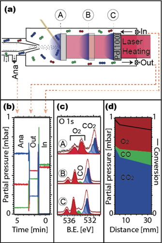
Figure 3. Gas-phase measurements above a catalytic active surface in the mass transfer limit at different heights above the surface. (a) Measurement geometry with the sample–cone distances of 0.6 mm, 5.6 mm, and 33.6 mm, respectively. (b) MS signals for 0.6 mm sample–cone distance. (c) O 1s spectra measured for each sample–cone distance. (d) Partial pressure calculated from the O 1s spectra in panel (c).
Download figure:
Standard image High-resolution imageTo map the spatial distribution of the gas composition orthogonal to the sample surface we retracted it stepwise from the aperture while measuring the gas phase O 1s spectra at each position (see panels (a) and (c) of figure 3). As the total pressure in the cell is 1 mbar it is straightforward to convert the peak areas of the different gas phase components in panel (c) to real partial pressures. They are shown in panel (d). Inspection of partial pressures now spatially resolved orthogonal to the sample surface in panel (d) confirms that the size of the mass transfer-limited zone extends ∼5 mm out from the surface with a step gradient of the CO pressure. We therefore conclude that the aperture of the electron analyser always will be located well within the CO depletion layer if positioned one or two diameters away from the sample surface at typical reaction conditions in APXPS setup. Furthermore, we note that this conclusion even will be valid in a back-filled setup as a zone with mass transfer limitation also will be formed in this case.
That the aperture of the electron analyser is well within the CO depletion layer fits well with the conclusions reached in combined planar laser-induced fluorescence (PLIF) and APXPS studies. The first of these (Blomberg et al 2016) compared PLIF and APXPS results for CO oxidation over Pd(100), and more recently an APXPS model reactor was studied solely with PLIF (Zhou et al 2017). In this recent study the authors built a nozzle-based PLIF setup to mimic a real APXPS setup. One important take-home message from this study is that the gas composition measured by PLIF in the vicinity of the sample differs substantially from that measured by mass spectrometry through a 1 mm nozzle placed 2 mm above the sample surface. For the case discussed above, a closer comparison of panels (b) and (d) in figure 3 shows, however, quite good agreement between the partial pressure of CO2 of 0.62 mbar measured with the MS and the 0.68 mbar estimated from the APXPS gas phase spectra, matching well with the expected number for 100% conversion 0.67 mbar.
4. Catalysis
As is seen from figure 2 catalysis is the field of science that makes most frequent use of APXPS. With respect to catalysis, one needs to distinguish between liquid phase catalysis (which includes most of the catalytic reactions of homogeneous catalysis) and vapour phase catalysis, in which the catalytic reaction typically takes place at the interface between a solid surface and the reactant vapour (i.e. it mostly addresses heterogeneous catalysis). That APXPS is particularly strong in the field of vapour phase/heterogeneous catalysis is not very surprising, given the strong linkage of surface science and catalysis in general and of XPS and catalytic investigations in particular. The mere fact that heterogeneous catalysis is concerned with the control of surface reactions and the interaction of vapour with solids makes the field predestined for APXPS.
Table 1. Catalytic reactions that have been studied by APXPS. Only studies carried out at a minimum pressure of 1 × 10⁻³ mbar have been included.
| Sample | Model catalyst | Gases | Maximum pressure during catalytic reaction (mbar) | Temperature in catalytic reaction (K) | Year | References |
|---|---|---|---|---|---|---|
| Alcohol oxidation | ||||||
| CeO2(100) | X | CH3OH, O2 | 0.4 | 520–720 | 2018 | Mullins (2018) |
| Co(0001) | X | CH3OH, O2 | 0.3 | 520 | 2010 | Zafeiratos et al (2010b) |
| Cu foil | X | CH3OH, O2 | 0.1 | 420–670 | 2003 | Bukhtiyarov et al (2003), |
| Prosvirin et al (2003) | ||||||
| Cu foil | CH3OH, O2 | 0.6 | 670 | 2004 | Bluhm et al (2004) | |
| Cu foil | CH3OH, O2 | 0.1 | 300–670 | 2016 | Prosvirin et al (2016) | |
| Pd nanoparticles | CH3OH, O2 | 0.5 | 300–390 | 2015 | Jürgensen et al (2015) | |
| on TiO2 catalyst | ||||||
| Pd(111) | X | CH3OH, O2 | 0.03 | 300–6000 | 2012 | Kaichev et al (2012) |
| Pt(111) | X | CH3OH, O2 | 0.02 | 340–500 | 2013 | Miller et al (2013), |
| Kaichev et al (2014b) | ||||||
| PtCo nanoparticles | X | CH3OH, O2 | 0.3 | 520 | 2012 | Papaefthimiou et al (2012) |
| supported on TiO2 | ||||||
| PtRe surface alloy | X | CH3OH, O2 | 0.4 | 300–550 | 2015 | Duke et al (2015b) |
| Re film supported on Pt(111) | X | CH3OH, O2 | 0.4 | 300–500 | 2015 | Duke et al (2015b) |
| RuO2(110)/Ru(0001) | X | CH3OH, O2 | 0.2 | 400–540 | 2007 | Blume et al (2007a), |
| Blume et al (2007b) | ||||||
| SrTiO3(100) | X | CH3OH, O2; | 0.3 | 370–570 | 2017 | Zhang et al (2017) |
| CH3CH2OH, O2 | ||||||
| V2O5/TiO2 catalyst | CH3OH, O2 | 0.25 | 370–470 | 2014 | Kaichev et al (2014a) | |
| Alcohol steam reforming | ||||||
| CeO2 microparticles | CH3CH2OH, H2O | 1.5 | 620–720 | 2016 | Sohn et al (2016) | |
| CeO2 nanoparticles | CH3CH2OH, H2O | 1.5 | 620–720 | 2016 | Sohn et al (2016) | |
| CeO2(111) supported | X | CH3CH2OH, H2O | 0.3 | 300–700 | 2016 | Liu et al (2016b) |
| on Ru(0001) | ||||||
| Co nanoparticles | CH3CH2OH, H2O | 0.3 | 670 | 2016 | Turczyniak et al (2016) | |
| supported on ZnO nanowires | ||||||
| Co(0001) | X | CH3CH2OH, H2O | 0.3 | 520 | 2016 | Turczyniak et al (2016) |
| Co/CeO2 catalyst | X | CH3CH2OH, H2O | 0.3 | 690 | 2016 | Turczyniak et al (2016) |
| Co/CeO2 microparticles | CH3CH2OH, H2O | 1.5 | 620–720 | 2016 | Sohn et al (2016), | |
| Sohn et al (2017) | ||||||
| Co/CeO2 nanoparticles | CH3CH2OH, H2O | 1.5 | 620–720 | 2016 | Sohn et al (2016), | |
| Sohn et al (2017) | ||||||
| Co2O3 nanoparticles | CH3CH2OH, H2O | 0.3 | 620 | 2016 | Turczyniak et al (2016) | |
| Ga/Pd foil | X | CH3OH, H2O | 0.4 | 420–670 | 2012 | Rameshan et al (2012b) |
| In/Pd foil | X | CH3OH, H2O | 0.2 | 330–650 | 2012 | Rameshan et al (2012a) |
| Ni/CeO2(111) | X | CH3CH2OH, H2O | 0.3 | 300–700 | 2016 | Liu et al (2016b) |
| supported on Ru(0001) | ||||||
| NiZn catalyst | CH3OH, H2O | 0.2 | 690 | 2012 | Friedrich et al (2012a) | |
| PdZn catalyst | CH3OH, H2O | 0.5 | 300–690 | 2012 | Friedrich et al (2012b) | |
| PdZn catalyst | CH3OH, H2O | 0.5 | 520 | 2012 | Halevi et al (2012) | |
| PdZn/Pd(111) | X | CH3OH, H2O | 0.4 | 300–620 | 2010 | Rameshan et al (2010a), |
| Rameshan et al (2010b) | ||||||
| Pt/In2O3/Al2O3 | CH3OH, H2O | 0.2 | 520 | 2013 | Barbosa et al (2013) | |
| PtCo foil | CH3OH, H2O | 0.5 | 750 | 2010 | Zafeiratos et al (2010a) | |
| PtCo nanoparticles | X | CH3OH, H2O | 0.3 | 520 | 2012 | Papaefthimiou et al (2012) |
| supported on TiO2 | ||||||
| PtRuCo catalyst | CH3OH, H2O | 0.5 | 750 | 2010 | Zafeiratos et al (2010a) | |
| RdPd/CeO2 catalyst | CH3OH, H2O | 0.05 | 820 | 2014 | Divins et al (2014) | |
| RhPd nanoparticles | CH3OH, H2O | 0.05 | 820 | 2014 | Divins et al (2014) | |
| Zn/Cu | CH3OH, H2O | 0.4 | 300–690 | 2012 | Rameshan et al (2012c) | |
Table 1. Continued.
| Sample | Model catalyst | Gases | Maximum pressure during catalytic reaction (mbar) | Temperature in catalytic reaction (K) | Year | References |
|---|---|---|---|---|---|---|
| Alcohol steam reforming, oxidative | ||||||
| Ga/Pd foil | X | CH3OH, H2O, O2 | 0.25 | 300–620 | 2012 | Rameshan et al (2012b) |
| Aldehyde hydrogenation | ||||||
| Pd film supported on Cr/SiO2 | Furan-2-aldehyd, H2 | 0.8 | 360 | 2014 | Pang et al (2014) | |
| coated with 1-octadecanethiol | ||||||
| Pd film supported on Cr/SiO2 | Furan-2-aldehyd, H2 | 0.8 | 360 | 2014 | Pang et al (2014) | |
| coated with benzene-1, | ||||||
| 2-dithiol (BDT) | ||||||
| Alkane dehydrogenation | ||||||
| CNT | Butane, O2 | 0.3 | 620–650 | 2008 | Zhang et al (2008) | |
| CNT | Butane, O2 | 0.3 | 650 | 2018 | Qi et al (2018) | |
| Pt/Mg(Al)O, PtSn/Mg(Al)O | C2H6, H2, O2, H2O | 1 | 300–450 | 2007 | Virnovskaia et al (2007) | |
| Alkane isomerisation | ||||||
| PtRh nanoparticles | H2, hexane | 0.2 | 300–630 | 2013 | Musselwhite et al (2013) | |
| Alkane oxidation | ||||||
| Co3O4/CeO2 | CH4, O2 | 1.6 | 420–820 | 2018 | Dou et al (2018) | |
| MoVOx | C3H8, O2, H2O | 0.3 | 540 | 2017 | Trunschke et al (2017) | |
| MoVTeNb | C3H8, O2, H2O, He | 0.3 | 320–690 | 2012 | Hävecker et al (2012) | |
| MoVTeNbOx | C3H8, C3H6, O2, H2O | 0.3 | 623 | 2010 | Sanfiz et al (2010) | |
| Ni foil | C3H8, O2 | 2.0 | 870–970 | 2013 | Kaichev et al (2013) | |
| NiCo2O4 | CH4, O2 | ∼1.0 | 300–670 | 2015 | Tao et al (2015) | |
| NiFe2O4 | CH4, O2 | 0.8 | 300–670 | 2016 | Zhang et al (2016) | |
| NiO/CeO2 | CH4, O2 | 1.6 | 420–770 | 2018 | Zhang et al (2018a) | |
| Pd(100) | X | CH4, O2 | 0.7 | 440–770 | 2014 | Martin et al (2014) |
| Pd(111) | X | CH4, O2 | 0.33 | 415–815 | 2007 | Bluhm et al (2007) |
| Pd(111) | X | CH4, O2 | 0.3 | 420–850 | 2007 | Gabasch et al (2007) |
| Pd, Pt, Rh/CeO2 | X | CH4, O2 | 4.0 | 300–870 | 2013 | Zhu et al (2013a) |
| Pd/Al2O3 | CH4, O2 | 0.1 | 570 | 2013 | Stakheev et al (2013) | |
| Pd/Al2O3 | CH4, O2 | 0.3 | 400–700 | 2016 | Price et al (2016) | |
| Pd/Al2O3 | C3H8, O2 | 0.02 | 620–720 | 2017 | Khudorozhkov et al (2017) | |
| Pt/Al2O3 | CH4, O2 | 0.02 | 680–780 | 2016 | Pakharukov et al (2016) | |
| (VO)2P2O7 | n-C4H10, O2, He | 2.0 | 520–670 | 2003 | Hävecker et al (2003) | |
| (VO)2P2O7 | n-C4H10, O2, He | 2.0 | 420–670 | 2005 | Kleimenov et al (2005) | |
| (VO)2P2O7 | n-C4H10, O2, He | 0.5 | 370–670 | 2012 | Eichelbaum et al (2012) | |
| (VO)2P2O7 | C3H8, O2, H2O, He | 0.3 | 670 | 2018 | Heenemann et al (2018) | |
| V2O5, MoVTeNbOx | C4H10, O2, He | 0.3 | 670 | 2015 | Eichelbaum et al (2015) | |
| Alkane oxidation, wet | ||||||
| MoVTeNb | C3H8, O2, H2O, He | 0.3 | 320–690 | 2012 | Hävecker et al (2012) | |
| Alkene oxidation | ||||||
| Ag nanopowder | C2H4, O2 | 0.3 | 500 | 2014 | Rocha et al (2014) | |
| Ag NP/alumina | C3H6, O2 | 0.5 | 470 | 2010 | Lei et al (2010) | |
| Ag/HOPG | X | C2H4, O2 | 0.3 | 350–470 | 2011 | Demidov et al (2011a) |
| Ag/HOPG | X | C2H4, O2 | 0.5 | 420–480 | 2011 | Demidov et al (2011b) |
| CuAg nanopowder | C2H4, O2, H2 | 0.5 | 520 | 2010 | Piccinin et al (2010) | |
| Pd(111) | X | C2H4, O2 | 2 × 10⁻³ | 330–923 | 2006 | Gabasch et al (2006) |
| Pd(551) | X | C3H6, O2 | 0.5 | 370–570 | 2018 | Kaichev et al (2018) |
| Ag foil | X | C2H4, O2 | 0.6 | 370–520 | 2006 | Bukhtiyarov et al (2006) |
| Alkene hydrogenation | ||||||
| Pd foil | 1-Pentene, propene, | 1.0 | 350 | 2008 | Teschner et al (2008a) | |
| acetylene, H2 | ||||||
| Pd(111) and Pd foil | X | trans-2-Pentene, H2 | 0.8 | 300–520 | 2005 | Teschner et al (2005) |
| PdGa pills | C2H2, H2 | 1.1 | 400 | 2009 | Kovnir et al (2009) | |
Table 1. continued.
| Sample | Model catalyst | Gases | Maximum pressure during catalytic reaction (mbar) | Temperature in catalytic reaction (K) | Year | References |
|---|---|---|---|---|---|---|
| Alkyne hydrogenation | ||||||
| PdGa, Pd/silica | C2H2, H2 | 1.1 | 300 | 2007 | Kovnir et al (2007) | |
| PtFe NP/SiO2 | C2H4, H2 | 0.2 | 300 | 2016 | Wang et al (2013b) | |
| Al13Fe4(010) | X | C2H2, H2 | 1.1 | 470 | 2012 | Armbrüster et al (2012) |
| Cu60Pd40 pills | C2H2, H2 | 1.1 | 390 | 2013 | Friedrich et al (2013) | |
| CuNiFe, CuFe pellets | C3H4, H2 | 2.0 | 523–783 | 2011 | Bridier et al (2011) | |
| InPd2 pills | C2H2, H2 | 1.0 | 470 | 2016 | Luo et al (2016) | |
| Pd black, Pd foil | C2H2, propyne, | 7.5 | 300–350 | 2008 | Teschner et al (2008b) | |
| 1-pentyne | ||||||
| Pd CNT, Pd(111), Pd foil | X | 1-pentyne, | 0.9 | 360–520 | 2006 | Teschner et al (2006a) |
| trans-2-Pentene, H2 | ||||||
| Pd foil, Pd CNT | C3H4, H2 | 1.1 | 350–390 | 2010 | Teschner et al (2010) | |
| PdGa NPs/CNT | C2H2, H2 | 1.1 | 390 | 2011 | Shao et al (2011) | |
| Ammonia decomposition | ||||||
| Ni(111) | X | NH3 | 0.6 | 300 805 | 2017 | Zhong et al (2017) |
| Pt(111) | X | NH3 | 0.6 | 300–840 | 2017 | Zhong et al (2017) |
| Pt/Ni/Pt(111) | X | NH3 | 0.6 | 300–800 | 2017 | Zhong et al (2017) |
| Ammonia oxidation | ||||||
| Pt(533) | X | NH3, O2 | 1.0 | 340–770 | 2007 | Imbihl et al (2007), |
| Günther et al (2008) | ||||||
| CO oxidation | ||||||
| Au nanoparticles evaporated | X | CO, O2 | 1.0 | 300 | 2012 | Dumbuya et al (2012) |
| onto TiO2(110) | ||||||
| Au nanoparticles on SiO2 and | CO, O2 | 0.3 | 420 | 2009 | Herranz et al (2009) | |
| TiO2 powder | ||||||
| Au nanoparticles supported on Au foil | X | CO, O2 | 0.3 | 300 | 2016 | Klyushin et al (2016) |
| Au nanoparticles supported on HOPG | X | CO, O2 | 0.3 | 300 | 2016 | Klyushin et al (2016) |
| Au/TiO2 powder catalyst | CO, O2 | 1.0 | 300–350 | 2006 | Willneff et al (2006) | |
| AuPd nanoparticles | CO, O2 | 0.4 | 370 | 2011 | Alayoglu et al (2011) | |
| Co3O4 nanoparticles | CO, O2 | 1.9 | 330–490 | 2018 | Tang et al (2018) | |
| Co3O4 nanorods | CO, O2 | 0.1 | 300–400 | 2017 | Jain et al (2017a), | |
| Jain et al (2017b) | ||||||
| CoO(100)/Ag(100) | X | CO, O2 | 1.2 | 300–550 | 2017 | Urpelainen et al (2017) |
| CoPt nanoparticles | CO, O2 | 1.1 | 400 | 2012 | Zheng et al (2012) | |
| Cu(111) | X | CO, O2 | 0.04 | 300 | 2014 | Xu et al (2014) |
| Cu0.1Ce0.9O2−x nanoparticles | CO, O2 | 0.1 | 570 | 2017 | Elias et al (2017) | |
| Ir(111) | X | CO, O2 | 0.5 | 300–575 | 2017 | Johansson et al (2017a) |
| Nanoporous Au containing | X | CO, O2 | 1.0 | 300 | 2009 | Wittstock et al (2009) |
| Ag impurities | ||||||
| Pd(100) | X | CO, O2 | 0.3 | 300–640 | 2012 | Toyoshima et al (2012b) |
| Pd(100) | X | CO, O2 | 0.7 | 420–680 | 2013 | Blomberg et al (2013) |
| Pd(100) | X | CO, O2 | 1.3 | 300–710 | 2016 | Blomberg et al (2016) |
| Pd(100) | X | CO, O2 | 0.7 | 350–500 | 2016 | Fernandes et al (2016) |
| Pd(110) | X | CO, O2 | 0.3 | 300–560 | 2013 | Toyoshima et al (2013) |
| Pd(111) | X | CO, O2 | 0.8 | 470–670 | 2012 | Toyoshima et al (2012a) |
| Pd(111) | X | CO, O2 | 0.1 | 350 | 2015 | Gopinath et al (2015), |
| Roy et al (2016) | ||||||
| Pd(111) modified by O implantation | X | CO, O2 | 0.1 | 350 | 2015 | Gopinath et al (2015), |
| Roy et al (2016) | ||||||
| Pd(111), curved | X | CO, O2 | 0.6 | 485–560 | 2018 | Schiller et al (2018) |
| Pd3Au(100) | X | CO, O2 | 1.0 | 300–600 | 2017 | Strømsheim et al (2017) |
| Pd75Ag25(100) | X | CO, O2 | 0.7 | 330–710 | 2016 | Fernandes et al (2016) |
| Pd7Au3(111) | X | CO, O2 | 0.1 | 300–570 | 2017 | Toyoshima et al (2017) |
Table 1. Continued.
| Sample | Model catalyst | Gases | Maximum pressure during catalytic reaction (mbar) | Temperature in catalytic reaction (K) | Year | References |
|---|---|---|---|---|---|---|
| Pt nanoparticles | CO, O2 | 1.0 | 370 | 2017 | Artiglia et al (2017) | |
| on CeO2 powder | ||||||
| Pt nanoparticles | CO, O2 | 2.7 | 500 | 2018 | Bergman et al (2018) | |
| supported on Al2O3 powder | ||||||
| Pt nanoparticles | CO, O2 | 0.2 | 470–520 | 2013 | An et al (2013) | |
| supported on mesoporous CeO2 | ||||||
| Pt nanoparticles | CO, O2 | 0.2 | 470–520 | 2013 | An et al (2013) | |
| supported on mesoporous MnO2 | ||||||
| Pt nanoparticles | CO, O2 | 3.0 | 370–540 | 2018 | Vakili et al (2018) | |
| supported on MOFs | ||||||
| Pt nanoparticles | CO, O2 | 1.0 | 300–600 | 2017 | Krick Calderón et al (2017) | |
| supported on TiO2 nanorods | ||||||
| Pt nanoparticles | X | CO, O2 | 1.0 | 300–450 | 2018 | Naitabdi et al (2018) |
| supported on TiO2(110) | ||||||
| Pt(110) | X | CO, O2 | 0.5 | 300–420 | 2009 | Chung et al (2009) |
| Pt(110) | X | CO, O2 | 0.5 | 790–840 | 2017 | Yu et al (2017) |
| Pt(111) | X | CO, O2 | 0.2 | 450–540 | 2012 | Schnadt et al (2012) |
| Pt(111) | X | CO, O2 | 0.7 | 300–550 | 2015 | Duke et al (2015a) |
| Pt(111) | X | CO, O2 | 1.0 | 300–1020 | 2016 | Krick Calderón et al (2016) |
| Pt(111) | X | CO, O2 | 0.2 | 415–535 | 2016 | Knudsen et al (2016) |
| Pt(111) | X | CO, O2 | 0.3 | 450–535 | 2017 | Johansson et al (2017a) |
| Pt3Ni(111) | X | CO, O2 | 0.2 | 300–540 | 2018 | Kim et al (2018) |
| Pt3Sn(111) | X | CO, O2 | 0.6 | 300–570 | 2012 | Jugnet et al (2012) |
| Pt3Ti polycrystal | X | CO, O2 | 1.1 | 300–370 | 2016 | Jeong et al (2016) |
| PtCu nanocubes | CO, O2 | No detailed | 300–480 | 2017 | Shan et al (2017) | |
| information | ||||||
| PtSn nanoparticles | CO, O2 | 0.2 | 550–640 | 2014 | Michalak et al (2014) | |
| PtZn nanoparticles | X | CO, O2 | 1.0 | 300–450 | 2018 | Naitabdi et al (2018) |
| supported on TiO2(110) | ||||||
| Rh nanoparticles | CO, O2 | 0.6 | 370–550 | 2008 | Grass et al (2008) | |
| Rh(100) | X | CO, O2 | 1.3 | 370–730 | 2014 | Gustafson et al (2014) |
| RhPd nanoparticles | CO, O2 | 0.3 | 450 | 2011 | Renzas et al (2011) | |
| RhPt alloy on Pt(111) | X | CO, O2 | 0.7 | 300–500 | 2015 | Duke et al (2015a) |
| Ru nanoparticles | CO, O2 | 0.4 | 320–370 | 2012 | Qadir et al (2012) | |
| Ru polycrystalline film | CO, O2 | 0.4 | 320–470 | 2013 | Qadir et al (2013) | |
| Ru(0001) | X | CO, O2 | 0.1 | 350–590 | 2006 | Blume et al (2006) |
| Ru(0001) | X | CO, O2 | 1.0 | 370–600 | 2007 | Bluhm et al (2007) |
Ru(10 ) ) | X | CO, O2 | 0.3 | 370–520 | 2014 | Toyoshima et al (2014) |
| TiCuOx on Cu(111) | X | CO, O2 | 0.05 | 300 | 2014 | Baber et al (2014) |
| TiO2/Au(111) | X | CO, O2 | 0.3 | 300–400 | 2017 | Palomino et al (2017a) |
| Zn nanoparticles | X | CO, O2 | 1.0 | 300–450 | 2018 | Naitabdi et al (2018) |
| supported on TiO2(110) | ||||||
| CO oxidation, wet | ||||||
| Co3O4 nanorods | CO, O2, H2O | 0.1 | 300–400 | 2017 | Jain et al (2017a), Jain et al (2017b) | |
| CO oxidation by water | ||||||
| Ag nanoparticles on TiO2(101) | X | CO, H2O | 3.0 | 300 | 2017 | Wagstaffe et al (2017) |
| CO oxidation, preferential in hydrogen | ||||||
| CeO2-promoted Co3O4 catalyst | CO, O2, H2 | 0.5 | 570 | 2016 | Lukashuk et al (2016) | |
| Co3O4−x nanorods | CO, O2, H2 | 1.0 | 300–410 | 2015 | Nguyen et al (2015) | |
| Pd/CeO2 catalyst | CO, O2, H2 | 0.5 | 358–523 | 2006 | Pozdnyakova et al (2006a) | |
| Pt on Co3O4−x nanorods | CO, O2, H2 | 1.0 | 300–410 | 2015 | Nguyen et al (2015) | |
| Pt/CeO2 catalyst | CO, O2, H2 | 0.5 | 358–523 | 2006 | Pozdnyakova et al (2006b), | |
| Teschner et al (2006b) | ||||||
| Pt/CeO2 catalyst | CO, O2, H2 | 1.0 | 393 | 2007 | Teschner et al (2007) | |
| PtSn catalyst | CO, O2, H2 | 0.7 | 393–473 | 2012 | Teschner et al (2012) | |
Table 1. Continued.
| Sample | Model catalyst | Gases | Maximum pressure during catalytic reaction (mbar) | Temperature in catalytic reaction (K) | Year | References |
|---|---|---|---|---|---|---|
| CO and CO2 hydrogenation in H2 | ||||||
| Co foil | CO, H2 | 0.1 | 520 | 2017 | Wu et al (2017) | |
| Co3O4 nanoparticles | CO, H2 | 0.4 | 500 | 2016 | Alayoglu and Somorjai (2016) | |
| supported on MgO nanoplates | ||||||
| Co3O4 nanorods, | CO2, H2 | 0.7 | 300–690 | 2012 | Zhu et al (2012) | |
| undoped and Ru-doped | ||||||
| CoRh nanoparticles | CO, H2 | 0.1 | 500 | 2016 | Liu et al (2016a) | |
| Cu(111) | X | CO2, H2 | 1.2 | 300–650 | 2018 | Ren et al (2018) |
| Cu/CeO2 catalyst | CO2, H2 | 0.06 | 300–720 | 2018 | Lin et al (2018) | |
| CuCo nanoparticles | CO, H2 | 0.5 | 370–520 | 2013 | Carenco et al (2013) | |
| Fe2O3, unpromoted and | CO, H2 | 0.4 | 550–620 | 2010 | de Smit et al (2010) | |
| promoted with Cu and Cu/K/Si | ||||||
| Mesoporous NiO | CO2, H2 | 5.0 | 573–673 | 2018 | Sápi et al (2018) | |
| MnO catalyst | CO, H2 | 0.7 | 670 | 2017 | Zhu et al (2017) | |
| MnO nanoparticles | CO, H2 | 0.4 | 500 | 2016 | Ralston et al (2016) | |
| supported on mesoporous Co3O4 | ||||||
| Ni(110) | X | CO, H2; CO2 H2; | 0.1 | 425 | 2016 | Roiaz et al (2016) |
| CO, CO2, H2 | ||||||
| Ni(111) | X | CO2, H2 | 0.5 | 300–570 | 2016 | Heine et al (2016) |
| NiCo nanoparticles | CO, H2 | 0.3 | 300–420 | 2015 | Carenco et al (2015) | |
| Pd(111) (ion bombarded) | X | CO, H2 | 0.1 | 300 | 2004 | Rupprechter et al (2004) |
| Pt nanoparticles | CO2, H2 | 5.0 | 573–673 | 2018 | Sápi et al (2018) | |
| supported on mesoporous NiO | ||||||
| Ru nanoparticles | CO, H2 | 0.7 | 300–420 | 2014 | Martínez-Prieto et al (2014) | |
| ZnO/Cu(100) and | X | CO2, H2 | 0.8 | 300–575 | 2018 | Palomino et al (2018) |
| ZnO/Cu(111) | ||||||
| RuO2 nanoparticles supported | X | CO2, H2 | 0.3 | 300–470 | 2016 | Carenco et al (2016) |
| on TiO2 on Au | ||||||
| RuO2 nanoparticles supported | CO2, H2 | 0.3 | 300–470 | 2016 | Carenco et al (2016) | |
| on TiO2 on powder | ||||||
| CO2 photoreduction | ||||||
| Pt/TiO2/mesoporours | CO2, H2O | 0.05 | 300 | 2018 | Tasbihi et al (2018) | |
| silica | ||||||
| CO2 reduction by water | ||||||
| Cu(111) | X | CO2, H2O | 0.9 | 300 | 2017 | Favaro et al (2017) |
| Co foil | CO2, H2O | 0.9 | 300 | 2018 | Liu et al (2018) | |
| Cross-coupling reactions | ||||||
| Au(111) | X | Ethynylbenzene, | 0.2 | 310–530; | 2017 | Johansson et al (2017b) |
| chlorobenzene; | 310–720 | |||||
| ethynylbenzene, | ||||||
| iodobenzene | ||||||
| Hydrogen–deuterium exchange | ||||||
| Pt(111) | X | H2, D2, CO | 0.3 | 300–480 | 2006 | Montano et al (2006) |
| Hydrodeoxygenation | ||||||
| Fe2O3 catalyst | 3-Methylphenol, H2 | 0.5 | 570 | 2017 | Hong et al (2017) | |
| Mo2C/SiO2 catalyst | Methoxybenzene, H2 | 1.0 | 590 | 2018 | Murugappan et al (2018) | |
| MoO3/SiO2 catalyst | Methoxybenzene, H2 | 1.0 | 590 | 2018 | Murugappan et al (2018) | |
| Pd/Fe2O3 catalyst | 3-Methylphenol, H2 | 0.5 | 570 | 2017 | Hong et al (2017) | |
| H2 oxidation | ||||||
| Pt(557) | X | H2, O2 | 1.3 | 300 | 2013 | Zhu et al (2013b) |
| Methane dry reforming | ||||||
| Co,Ni, Cu/CeO2(111) | X | CH4, CO2 | 0.7 | 300–700 | 2017 | Liu et al (2017) |
Table 1. Continued.
| Sample | Model catalyst | Gases | Maximum pressure during catalytic reaction (mbar) | Temperature in catalytic reaction (K) | Year | References |
|---|---|---|---|---|---|---|
| Co/CeOx | CH4, CO2 | 0.2 | 300–820 | 2018 | Zhang et al (2018b) | |
| Ni(111) | X | CH4, CO2 | 0.5 | 300–900 | 2016 | Yuan et al (2016) |
| Ni/CeO2 | CH4, CO2 | 0.7 | 920 | 2008 | Gonzalez-DelaCruz et al (2008) | |
| PtCo/CeO2 | CH4, CO2 | 0.05 | 820 | 2018 | Xie et al (2018) | |
| ZrO2/Pt(111) | X | CH4, CO2 | 0.2 | 673–873 | 2018 | Rameshan et al (2018) |
| NO oxidation | ||||||
| Pt nanoparticles | NO, O2 | 2.7 | 500 | 2018 | Bergman et al (2018) | |
| supported on Al2O3 powder | ||||||
| NOx reduction, N2O reduction | ||||||
| Co3O4 nanorods | NO, CO | 5.3 | 300–500 | 2013 | Zhang et al (2013a) | |
| Ir(111) | X | NO, CO | 0.1 | 300–610 | 2016 | Ueda et al (2016) |
| Ir(111) | X | NO, CO | 0.4 | 300–520 | 2017 | Ueda et al (2017) |
| α-MnO2 nanorods | NO, CO | 2.7 | 300–750 | 2013 | Shan et al (2013) | |
| Pd1Com supported on | NO, H2 | 2.7 | 300–570 | 2016 | Nguyen et al (2016) | |
| Co3O4 nanorods | ||||||
| Pt1Com supported on | NO, H2 | 2.7 | 300–570 | 2016 | Nguyen et al (2016) | |
| Co3O4 nanorods | ||||||
| Rh atoms supported | NO, H2 | 2.7 | 300–570 | 2013 | Wang et al (2013a) | |
| on Co3O4 nanorods | ||||||
| Rh(111) | X | NO CO | 0.1 | 300–730 | 2018 | Ueda et al (2018) |
| Photocatalytic cleaning of oxides | ||||||
| TiO2/silicon | H2O, O2 | 1.1 | 290 | 2009 | Jribi et al (2009) | |
| Water–gas shift | ||||||
| Au nanoparticles encapsulated | CO, H2O | 2.0 | 400–540 | 2012 | Wen et al (2012) | |
| in mesoporous CeO2 | ||||||
| Au nanoparticles supported | CO, H2O | 2.0 | 400–540 | 2012 | Wen et al (2012) | |
| on CeO2 nanorods | ||||||
| Au/CeZrO4 | CO, H2O | 0.5 | 420–570 | 2007 | Goguet et al (2007) | |
| CeO2/CuO catalyst | CO, H2O | 0.6 | 470–520 | 2012 | Cámara et al (2012) | |
| CeOx nanoparticles | X | CO, H2O | 0.2 | 470–570 | 2013 | Mudiyanselage et al (2013) |
| supported on Cu(111) | ||||||
| Co3O4 nanorods | X | CO, H2O | No detailed | 380–570 | 2013 | Zhang et al (2013b) |
| information | ||||||
| CrO3/Fe2O3 catalyst | CO, H2O | 2.0 | 670 | 2016 | Keturakis et al (2016) | |
| Cu nanoparticles supported | CO, H2O | 1.1 | 580–720 | 2018 | Ma et al (2018) | |
| on Fe3O4 nanorods | ||||||
| CuO nanoparticles | CO, H2O | 1.3 | 460–650 | 2018 | Hou et al (2018) | |
| supported on Fe2O3 | ||||||
| Fe–Cu–Al–O catalyst | CO, H2O | 2.7 | 570–620 | 2013 | Ye et al (2013) | |
| Pd nanoparticles supported | CO, H2O | No detailed | 470–670 | 2015 | Shan et al (2015) | |
| on mesoporous MnO2 | information | |||||
| Pt nanoparticles encapsulated | CO, H2O | 2.0 | 400–540 | 2012 | Wen et al (2012) | |
| in mesoporous CeO2 | ||||||
| Pt nanoparticles supported | CO, H2O | 2.0 | 400–540 | 2012 | Wen et al (2012) | |
| on CeO2 nanorods | ||||||
| Pt nanoparticles supported | CO, H2O | No detailed | 520–570 | 2015 | Shan et al (2015) | |
| on mesoporous MnO2 | information | |||||
| Pt supported on multiwalled | CO, H2O | 0.6 | 300–520 | 2014 | Zugic et al (2014) | |
| carbon nanotubes, | ||||||
| with and without Na promoter | ||||||
| PtCo nanoparticles supported | X | CO, H2O | No detailed | 300–620 | 2013 | Zhang et al (2013b) |
| onCo3O4 nanorods | information | |||||
| PtRuCo catalyst | CO,H2O | 0.5 | 750 | 2010 | Zafeiratoset al (2010a) | |
Table 1 contains all APXPS studies of catalysis that we have been able to identify, categorised by the type of reaction, gases/vapours involved, maximum pressure during the catalytic reaction and temperature of the solid catalyst sample. The table follows the categorisation of Starr et al (2013), but in contrast to this earlier publication we have refrained from including all types of APXPS studies due to their sheer number. Of the identified catalysis studies around 45% are concerned with reactions on model catalysts, as indicated in table 1, and 55% on real catalysts. As model catalysts we have counted well-defined single crystals (as identified from the specification of Miller indices), typically prepared by UHV cleaning methods such as sputtering and annealing. In some cases, a well-defined surface can also be obtained from (flame) annealing or other preparation methods. Metal foils have been categorised as model catalysts if prepared by UHV sputter and anneal cycles. All other types of catalyst have been classified as 'real'. Naturally, such a definition of 'model catalyst' vs 'real catalyst' is quite arbitrary, given that many types of sample preparations could be considered as not representing a catalyst in its industrial or application state or form and hence to be a model. The definition has the virtue, however, of providing a clear-cut link to surface science experiments.
Real catalysts are often significantly more difficult to study than model catalysts. In particular, sample charging due to the emission of photoelectrons is an issue for insulating oxides and insulating oxide-supported catalytic nanoparticles. Studies of insulating and semiconducting materials are also hampered by the absence of a measurable Fermi level and thus the lack a natural binding energy reference. For only slightly insulating samples the situation can be remedied if care is taken to measure a reference spectrum directly prior or after the measurement of a new core or valence level. A determination of the photon energy and of the position of the low-energy secondary electron cut-off for the reference spectrum results in the possibility of referencing to the vacuum level, which is an appropriate reference level for insulators (Schnadt et al 2003). For more strongly insulating samples heating may remove the spectral shift due to charging (Price et al 2016). It has also been found that positively biasing of the insulating sample with some tens of volts can alleviate the problem (Boucly 2017). To our knowledge, electron guns for charge neutralisation, common for many standard XPS setups, are not yet available for the higher-pressure sample environments. A flood gun operating under the pressure conditions of APXPS would require a differential pumping stage not unlike that of an APXPS electron energy analyser.
As pointed out above, there exist many more reports of catalysis-related APXPS research than reported in table 1. We have included only such studies in table 1 in which the catalyst sample was exposed to catalytic conditions. Although highly relevant for catalysis, studies concerned with the exposure of the sample to one reactant only or with preparation routes have not been included. We have not included electrocatalysis studies (cf figure 2), either. Electrocatalysis is a field in its own right, with many exciting developments, a strong growth and its own experimental challenges.
From table 1 it is quite obvious that the study of fairly 'simple' chemical reactions such as the oxidation of carbon monoxide predominates in APXPS research, even today when the technique can be considered rather mature. Oxidation reactions are investigated much more frequently than hydrogenation reactions, not least because carbon contamination is significantly more difficult to fight in reducing than in oxidising conditions. The study of reactions involving larger molecules, of importance e.g. in relationship to the catalytic production of fine chemicals and pharmaceuticals, is hampered by the low vapour pressure of such compounds. Conventional APXPS relies on vapours with a sufficiently high pressure, and this precludes the study of many reactions of interest. It will be interesting to see whether flow cells, mentioned above, or liquid jet experiments will open for such investigations.
It is quite striking to consider the maximum pressures reported in the table 1. Although APXPS today can be done at much higher pressure (Kaya et al 2013, Schlueter et al 2019), essentially all studies limit themselves to the sub- to few-mbar range. Likely, the reason is that APXPS experiments still can be done with ease in this pressure range. The attenuation of both the x-rays and photoelectrons is not too severe and fair count rates of both the surface and gas phase signals can be achieved, without having to resolve to geometrically and mechanically very complicated instrument setups. Contamination, e.g. from the gases supplied to the solid sample, play an important role, but can also still be handled, for example by catalytic gas cleaning and liquid nitrogen traps. Moreover, the gas and surface signals are comparable in count rate at one mbar pressure, which is favourable for both the collection of data and their analysis. All these aspects change quite drastically at higher pressure and make the experiment considerably more difficult.
In the following we will discuss a few catalysis case studies that illustrate our ambition to turn our attention to more complex catalytic reactions. Starting from the CO oxidation on flat surfaces, we turn to the CO oxidation over structurally more complex, stepped surfaces. Then we discuss the preferential oxidation of CO in as CO/H2 mixture—in essence syngas—for which different reaction pathways achieved under different conditions play a fundamental role. Finally, we discuss the Sonogashira cross-coupling reaction, which is a catalytic C–C bond formation reaction of importance in the organic synthesis of complex molecules.
4.1. Complete oxidation: CO oxidation
While CO oxidation is extremely important in the three-way exhaust catalyst, it is not the most relevant process for industrial application in general. It is, however, a highly valuable probe reaction for surface catalysis reactions on metal surfaces, not least due to its relative simplicity. Only one reaction product, CO2, is possible, and only chemisorbed phases of CO/oxygen or surface oxides can exist on the catalyst surface. In addition, it is easy to keep surfaces clean at reaction conditions, as the oxidising environment typically removes carbon and other impurities, which segregate to the surface from the bulk of the crystal. Another advantage of the reaction are its high turn-over frequencies at relatively low temperature, which makes it easy to probe the reaction products in the gas phase. These properties of the CO oxidation reaction have made it one of the most popular model reactions to study with large variety of in situ techniques that recently have been developed.
Also with APXPS the CO oxidation has been studied extensively for a large number of transition metal polycrystalline and single crystal surfaces, as table 1 demonstrates. In fact the CO oxidation reaction is particular well suited for APXPS studies since (i) all gas phase reactants, products, adsorbed surface species, and the metal oxidation can be followed within the same spectrum, the O 1s spectrum, (ii) for almost all single crystal metal surfaces XP reference spectra of known surface structures of chemisorbed oxygen, CO, or metal oxides can be found in the literature, (iii) the high turn-over frequency makes the reaction particular well suited for APXPS which due to the pumping by the nozzle used to capture the photoelectrons makes every APXPS setup a continues flow cell.
In our first example we compare CO oxidation on the (111) facets of Pt and Ir (Johansson et al 2017a). Figures 4(a) and (d) compare O 1s spectra acquired on the Pt(111) and Ir(111) surfaces at stepwise increasing temperature in a 9:1 O2:CO mixture at a total pressure between 0.25 and 0.5 mbar. Starting with the components assigned to adsorbed species, we only observe adsorbed CO (blue components) at low temperature, with the CO molecules occupying bridge (CObridge) and atop (COatop) sites on Pt(111) and atop sites (COad) on Ir(111). Increasing the temperature, we observe components assigned to chemisorbed oxygen atoms (red components—Oad) formed by O2 dissociation on the two surfaces. Strong components assigned to O2 gas phase molecules (orange components O2a and O2b) are observed in both cases, while gas phase CO and CO2 are difficult to see as a result of the mixing ratio. The CO and CO2 signals are, however, easy to detect in the signal from the mass spectrometer coupled to the outlet of from the reactor cell of the APXPS setup (not shown, cf Johansson et al (2017a)). Judging the CO2 production as measured by the mass spectrometer, the CO covered surfaces are inactive, while the surfaces with chemisorbed oxygen are active with a clear production of gas phase CO2. Figures 4(b) and (d) displays the intensity of the CO and oxygen components together with the work function shift of the surface as probed by the shift of apparent binding energy of the O2 gas phase signal. Inspection of this figure reveals a striking difference between the two surfaces. While the transition on Pt(111) is sharp with either CO adsorbed or oxygen adsorbed, we observe co-adsorption phases of CO and oxygen in the temperature window between 450 and 550 K on Ir(111).
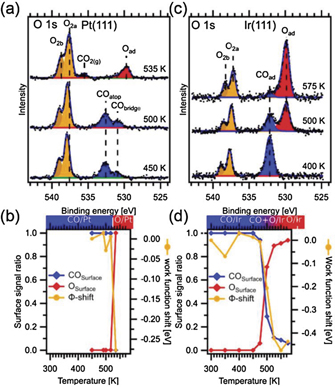
Figure 4. (a) O 1s APXP spectra acquired on Pt(111) in 9:1 O2:CO mixture at 0.2–0.5 mbar at stepwise increasing temperatures. (b) Corresponding intensity of the peaks assigned to surface species plotted together with the work function shift measured by the O2 gas phase signal. (c) and (d) Similar data for Ir(111). Reproduced from [Johansson N, Andersen M, Monya Y, Andersen J N, Kondoh H, Schnadt J and Knudsen J 2017a J. Phys.: Condens. Matter 29 444002]. © IOP Publishing Ltd. All rights reserved.
Download figure:
Standard image High-resolution imageTo explain why a sharp transition between CO- and oxygen-covered surfaces exist on Pt(111), while a 100 K wide co-existence regime is found for Ir(111), we need to go a step deeper and try to predict atomic-scale surface phases that exist near the switching point and in the transition region. To do this we first calculate the CO and oxygen coverage on the surface at each measurement temperature for the Ir(111) surface. We do this by curve fitting all relevant Ir 4f7/2 spectra, having components originating from Ir bulk atoms, Ir surface atoms, Ir surface atoms bound to CO atop, and Ir surface atoms bound to one or two O atoms in three-fold hollow sites simultaneously with correlated coefficients (i.e. only intensities are allowed to vary independently). Curve fitting is subject to the following constraints: (i) fixed probing depth and therefore a constant ratio between components assigned to Ir surface atoms and Ir bulk atoms; (ii) a ratio between COads and Oads that is consistent with the O 1s spectra of figure 4. As a result, we get the number of Ir surface atoms bound to no adsorbate, bound to CO atop, or bound to one or two O atoms, which automatically is normalised to one monolayer of Ir surface atoms. From these numbers it is straightforward to calculate the oxygen and CO coverage on the surface for each temperature which is shown figure 5.
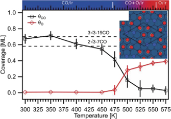
Figure 5. (a) Coverage of CO and oxygen for all measured temperatures on Ir(111). The inset in the top right corner shows the DFT-optimised structure that forms once adsorbed oxygen starts to deplete CO on the surface. Reproduced from [Johansson N, Andersen M, Monya Y, Andersen J N, Kondoh H, Schnadt J and Knudsen J 2017a J. Phys.: Condens. Matter 29 444002]. © IOP Publishing Ltd. All rights reserved.
Download figure:
Standard image High-resolution imageInspection of this figure reveals a coverage of ∼0.7 ML at 300 K fitting very well with the coverage a previously reported (3√3 × 3√3)R30° structure consisting of magic (CO)19 clusters. Increasing the temperature to 450 K the coverage drops to ∼0.55, which fits quite well with a previously reported (2√3 × 2√3)R30° structure with magic (CO)7 clusters. Once the temperature drops further, oxygen start to co-exist with the CO adsorbates. This suggest that the first transition structures are formed by removal of the weakest bound CO atoms in the (CO)7 clusters. In fact, DFT calculations show that O2 adsorption at our experimental conditions is highly favourable when two CO molecules are removed from each (CO)7 cluster (see inset of figure 5). Hence, the interplay of APXPS and DFT calculations suggests that a defected (2√3 × 2√3)R30° structure forms along with co-adsorbed O at the transition to the active phase for CO oxidation.
In a similar fashion one can find the CO and oxygen coverage at the different temperatures for the Pt(111) surfaces, deduce likely structures based on the known surface structures and use DFT calculations to predict whether or not O2 adsorption is favourable. In this case the combined APXPS and DFT work reveals that the CO coverage needs to be close to zero before O2 adsorption becomes favourable in good agreement with figure 4.
To conclude, this first case study shows that while a defective (2√3 × 2√3)R30° with only two CO molecules removed from each (CO)7 cluster favours O2 adsorption and dissociation on Ir(111) an almost CO-free surface is needed on Pt(111). The underlying reason for this striking difference can be explained by DFT calculations which provide evidence for an important difference between Ir and Pt:CO and O bind much more strongly to Ir than to Pt, and this is sufficient to overcome the repulsive CO–O interactions and to allow for mixed CO–O adsorbate structures on the Ir(111)surface. Another, important take-home message from this study is that within the transition region between the chemisorbed CO and oxygen phases low-coverage structures resembling those found at UHV conditions are likely to be formed, something which probably can be generalised to many other metal surfaces.
The second case study is focused on the transition state between a non-active and an active phase, i.e. a similar physical system is addressed as in the first case. The difference between the two studies is that Schiller et al (2018) in the second study used a cylindrical, curved Pd(111) crystal, which has (111) facets at the centre and (335) and (553) facets at each edge, respectively. This curvature gives rise two different types of step terminations: {111}-like (B-type) towards the (553) facet and {100}-like (A-type) towards the (335) facet. By scanning the small x-ray light spot (20 μm) across the curved crystal it becomes possible to probe how the different surface terminations affect the adsorbates and the catalytic performance at identical temperature and flow settings.
Figures 6(a) and (b) are reproduced from Schiller et al (2018). They display C 1s and O 1s spectra, respectively, as function of the vicinal angle, having the Pd(111) termination at 0°. These spectra were recorded using 0.3:0.3 mbar CO:O2 mixture, a total flow of 0.15 sccm, and a temperature of 485 K after cooling the sample from a temperature of 560 K. At 560 K the entire sample was in the mass transfer limit, with no adsorbed CO anywhere on the sample. In contrast, panel (a) clearly demonstrates that adsorbed CO in large quantities are present at the (111) facets, while the highly stepped surfaces found near the edges have much less adsorbed CO. Comparing the sides with A and B steps in the C 1s spectra it also becomes evident that the side with B-type steps is less poisoned by CO than the one with A-type steps. In the O 1s spectra shown in panel (b) a clear anti-correlation between adsorbed CO and the tail at right-hand side of the intense Pd 3p3/2 is observed. This tail is assigned to either chemisorbed oxygen or a Pd oxide. Panel (c) of figure 6 display the relative surface oxide intensity, obtained by carefully curve fitting the O 1s spectra of panel (b) while comparing with UHV spectra of CO and oxygen covered, and surface oxide covered Pd surfaces. Interestingly, inspection, of panel (c) reveals that Pd oxide patches are fully absent in the central region of the crystal, but abruptly grows beyond the the (557) and (443) facets. Based on this observation the authors suggest that the highly stepped surfaces beyond (557) and (443) facets are easier to oxidise and more difficult to reduce, which in turn leads to changed hysteresis behaviour when heating and cooling above and below the ignition temperature.
To conclude on the second case study, it demonstrates how curved crystals can be used to study a multitude of vicinal surfaces in situ at identical flow and temperature settings. A spatial variation of active and poisoning phases was observed at stationary conditions and it is suggested that a Pd surface oxide is more easily developed and more difficult to remove at the highly stepped B-type steps, compared to highly stepped A-type steps, while (111) facets with few steps are much more difficult to oxidise and easy to reduce if oxidised.
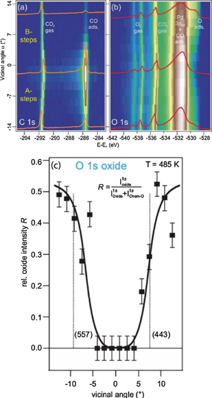
Figure 6. (a) C 1s and (b) O 1s measured across the curved crystal at 485 K. (c) Corresponding relative oxide intensity as function of the vicinal angle. Reprinted with permission from [Schiller F, Ilyn M, Pérez-Dieste V, Escudero C, Huck-Iriart C, Ruiz del Arbo N, Hagman B, Merte L R, Bertram F, Shipilin M, Blomberg S, Gustafson J, Lundgren E and Ortega J E 2018 J. Am. Chem. Soc. 140 16245]. Copyright (2018) American Chemical Society.
Download figure:
Standard image High-resolution image4.2. Preferential and partial oxidation: H2/CO oxidation
While the last example of section 4.1 used the introduction of step atoms to increase the complexity of model system we here discuss how one can study competing reactions with different reaction paths and hereby increase the complexity of the catalytic systems studied with APXPS. Such studies that go beyond a single reaction pathway are very important to mimic the often complex reaction conditions used for industrial catalysts. Here, we will use simultaneous CO and H2 oxidation as the simplest example of two competing reactions (cf previous studies by Nguyen et al (2015), Pozdnyakova et al (2006a), Nguyen et al (2015), Pozdnyakova et al (2006b), Teschner et al (2006a), Teschner et al (2007) and Teschner et al (2012)). Studying these two oxidation reactions simultaneously also have some technological relevance, as preferential oxidation of CO (PROX) is an important method for the removal of CO from hydrogen gas produced from fossil fuel.
Figure 7 shows simultaneous mass spectrometry data measured at the exhaust from the cell and APXPS data measured in front of the samples acquired while heating Pt(111) (a) and Ir(111) (b) surfaces with a constant heating rate of 9 K min−1. The surfaces where exposed to flows of 5 sccm O2, 0.5 sccm H2 and 0.5 sccm CO which resulted in a total pressure of about 0.5 mbar in the cell.
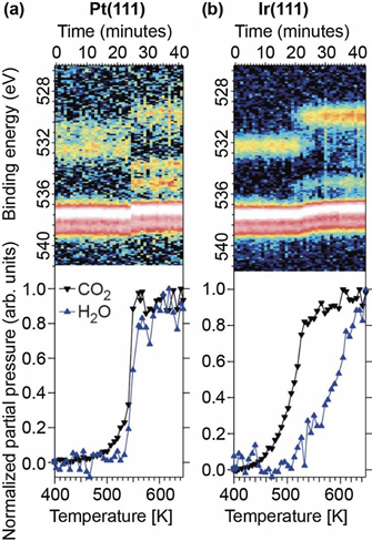
Figure 7. Mass spectrometry data and APXP spectra of the O 1s region collected simultaneously during a heating ramp of the substrates for (a) Pt(111) and (b) Ir(111), respectively.
Download figure:
Standard image High-resolution imageStarting with the data in panel (a) acquired on Pt(111) the situation is very similar to that observed during CO oxidation discussed above. Two regimes can be indentified: (i) a low activity regime below 550 K where no or very little H2O and CO2 are produced. (ii) A high activity regime above 550 K where H2O and CO2 are produced in large quantities. The fact that the H2O and CO2 production is constant and independent of temperature in the temperature interval from 550 to 650 K is clear evidence that both the H2 and CO oxidation reactions are mass transfer limited (MTL). The APXPS data reveals that the low-activity regime is dominated by adsorbed CO as identified by the two peaks above and below 532 eV assigned to CO adsorbed in top and bridge position, respectively. In the low-activity region only the O2 doublet (red/white colour in the figure) is observed in the gas phase signal. CO is not observed due to the gas mixing ratio: the large O2 doublet shadows the CO peak in the image plots. Changing to the high-activity regime the O2 doublet change position abruptly signalling a rapid change of the surface work function and CO2 (535.3 eV) and H2O (533.9 eV) are now clearly observed in the gas phase signal. At the surface both CO induced components disappeared and the surface is now dominated by a single peak at 529.8 eV assigned to chemisorbed oxygen. Based on these observations, it is clear that the Pt(111) surface change rapidly from a CO poisoned surface to an oxygen covered surface. The O-covered surface is very active both for CO and H2 oxidation and therefore immediately brings both reactions into the mass transfer limit.
Comparing the mass spectrometry data recorded for Ir(111), the situation is clearly different to the Pt(111) case. CO2 production increase rapidly in the temperature interval from ∼430 to ∼530 K and then continues to increase with slower rate. The CO2 production never becomes constants and the reaction therefore never reach the mass transfer limit for the CO oxidation reaction. H2O production first starts at ∼530 K and then increase up to the maximum temperature of 650 K. Thus, from the mass spectrometry data none of the reactions reach the mass transfer limit and it seems that the surface selectively oxidises CO at lower temperatures, while also H2 is oxidised above ∼530 K. Turning the O 1s APXP spectra image plot at the top of panel (b) it is clear that the surface is poisoned by atop-adsorbed CO, as signalled by a peak at 532 eV at low temperature. Once the CO molecules start to desorb, oxygen adsorbs on the surface, signalled by the peak 530 eV, and its coverage increases with temperature. During the entire active region the O2 doublet change peak position as observed by the 'bend' appearance in the image plot. Thus, the surface coverage change continuously within the active region fitting well with the fact CO and H2 oxidation never reach the MTL. Finally, we note that we almost exclusively observe CO2 production in the gas phase signal while the signal for H2O is just above the noise level.
From these observations we conclude that the oxidation of CO over Ir(111) proceeds much like in the case without H2 in the gas mixture with a slow change of the surface state from CO-covered to co-existing chemisorbed O and CO species and finally to surface dominated by adsorbed O-atoms. This slow change in surface state facilitates the PROX reaction. Or put differently, as we never reach the mass transfer limit CO must be present in small quantities in the gas atmosphere just above the sample. With both CO and H2 in the gas atmosphere just above the sample the surface much more efficiently oxidise CO. A similar situation is very difficult to achieve with Pt(111) as the sample rapidly change from fully CO covered to fully oxygen covered and directly jumps into the MTL.
4.3. Sonogashira cross-coupling
It remains a challenge for APXPS to study chemically more complex catalytic reactions, for example due to contamination issues, low vapour pressures of the reactants and complexity of the reaction mechanism. Here, we provide an example of a study in which a chemically more advanced catalytic reaction was investigated, namely the Sonogashira cross-coupling reaction (Sonogashira et al 1975, cf scheme
The Sonogashira reaction falls within the class of metal-catalysed cross-coupling reactions that lead to the formation of C–C bonds. Cross-coupling reactions are of superior importance in organic synthesis and are used in the fine chemical and pharmaceutical industry (Anastasia and Negishi 2002, Meijere and Diederich 2004, Wu et al 2010). The Sonogashira cross-coupling reaction is catalysed by gold nanoparticles (González-Arellano et al 2007). UHV studies by Sánchez-Sánchez et al (2014) and Kanuru et al (2010) suggest that also the Au(111) single crystal surface mediates the reaction. In an APXPS experiment (Johansson et al 2017b) we confirmed that this is the case also at pressures in the 10−1 mbar range; as will be seen in the following, we also find, however, that the elevated pressure conditions lead to a rapid inactivation of the Au(111) surface by a carbonaceous species.
In catalytic mixtures of a halobenzene (i.e. chlorobenzene or iodobenzene) and phenylacetylene the desired Sonogashira cross-coupling reaction competes with two other reactions. These are the Ullmann homocoupling reaction, in which two halobenzene molecules react to biphenyl (BP), and the homocoupling reaction between two phenylacetylene molecules to diphenyl diacetylene (DPDA), cf scheme
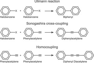
Scheme 1. Schemes of relevant coupling reactions. Reproduced from [Johansson N, Sisodiya S, Shayesteh P, Chaudhary S, Andersen J N, Knudsen J, Wendt O F and Schnadt J 2017b J. Phys.: Condens. Matter 29 444005]. © IOP Publishing Ltd. CC BY 3.0.
Download figure:
Standard image High-resolution imageThe spectral fingerprint of the desired DPA product can be identified from temperature-dependent UHV C 1s XPS data, cf the middle panel row of figure 8 with the data for the chlorobenzene/phenylacetylene reaction to the left and those for the iodobenzene/phenylacetylene reaction to the right in the figure. The spectra were acquired on a liquid nitrogen-cooled Au(111) sample, which was prepared by first adsorbing 0.7 (0.4) monolayers of chlorobenzene (iodobenzene), followed by adsorption of 0.4 monolayers of phenylacetylene. A combined temperature-programmed reaction and XPS study has shown previously that the Sonogashira cross-coupling reaction takes place at around −70 °C, while DPDA and BP are formed first above room temperature (Kanuru et al 2010). This identifies the low-energy component in the C 1s UHV XP spectra observed in the range between −65 °C and 5 °C and marked by the blue arrows as being related to DPA.
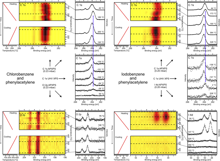
Figure 8. APXPS (total pressure 0.2 mbar) and UHV XPS results on the Sonogashira cross-coupling reaction on Au(111). The top and bottom row display the C 1s and halide APXP spectra, with the chlorobenzene/phenylacetylene cross-coupling reaction addressed to the left and the iodobenzene/phenylacetylene reaction to the right. For each of the two reactions a single heating and cooling cycle was carried out, and the APXP spectra in the image plots were acquired during the cycle. To the left of the image plots the temperature ramps are provided. The ramps differ somewhat between the C 1s and halogen spectra since the heating was continuous, while the APXP spectra were in an alternating fashion, switching back and forth between the C 1s and halogen regions. From the image plots APXP spectra were extracted at the indicated by the dashed lines. These spectra are shown to the right of the image plots. For comparison, the middle row displays UHV XPS spectra measured after dosing 0.4 monolayers of phenylacetylene on 0.7 (0.4) pre-adsorbed monolayers of chlorobenzene (iodobenzene). Reproduced from [Johansson N, Sisodiya S, Shayesteh P, Chaudhary S, Andersen J N, Knudsen J, Wendt O F and Schnadt J 2017b J. Phys.: Condens. Matter 29 444005]. © IOP Publishing Ltd. CC BY 3.0.
Download figure:
Standard image High-resolution imageThe corresponding APXPS data are shown in the top and bottom rows of figure 8. For both reactions, the chlorobenzene/phenylacetylene and the iodobenzene/phenylacetylene reaction, a heating and cooling cycle was carried out in the presence of a halobenzene/phenylacetylene 1:1 reaction mixture at a total pressure of 0.2 mbar. The APXPS data are shown as image plots, with the temperature ramp indicated to the left of the plots. In the panels to the right of each image plot single spectra are shown, which were extracted from the image plots at the indicated temperatures. The corresponding rows of the image plats are marked with dashed lines.
The surface adsorbates formed in the chemical reaction of the reactant vapours with the Au(111) surface give rise to the peaks located at around 284 eV in the C 1s spectra. The vapours induce the gas phase features at almost 285 eV binding energy, as can be easily identified from measurement on the gas phase in the absence of the sample surface. Similarly, the high binding energy doublet in the Cl 2p APXP spectra with the major component at 201.2 eV is due to the chlorobenzene gas phase, while the corresponding component at 52.5 eV in the I 4d spectra due to gas phase iodobenzene is barely visible.
The measurements were started at room temperature, and then the temperature was ramped up to a maximum of almost 300 °C for the chlorobenzene/phenylacetylene mixture and 450 °C for the iodobenzene/phenylacetylene mixture. In both cases a characteristic downshift of the C 1s line to the energy of DPA—as identified from the UHV XPS measurement—is seen, for the chlorobenzene reaction at around 170 to 190 °C and for iodobenzene in between approximately 100 to 220 °C. Hence, in this temperature range, and at a reactant pressure of around 0.2 mbar, the Sonogashira cross-coupling reaction takes place on the Au(111) surface. Further heating, however, leads to an upshift of the C 1s line, which is indicative of an inhibition of the DPA production. This line, with a binding energy of a little more than 284 eV, persists even upon cooling, and the activity towards DPA is not regained. Hence, the Au(111) is poisoned by a carbonaceous surface species.
The quasi-simultaneously measured halogen core levels give evidence of a difference between the chloro- and iodobenzene systems. The Cl 2p binding energy is indicative of exclusively non-dissociative adsorption of chlorobenzene on the Au(111) surface. In the I 4d APXP spectra two doublets are observed, which correspond to two different adsorbate species: a majority species with an I 4d5/2 component at around 48.4 eV binding energy and a minority species with an I 4d5/2 line at around 49.6 eV. These are identified with atomic iodine (and hence phenyl radicals) and intact iodobenzene, respectively. The difference in the halogen chemistry does not preclude the observation of the Sonogashira cross-coupling reaction for both chlorobenzene and iodobenzene.
We conclude that the Sonogashira cross-coupling reaction takes place over a Au(111) surface at moderate temperature and a processing pressure of around 0.2 mbar. This confirms earlier UHV results that Au(111) catalyses the reaction. What could not be seen in these UHV studies was the rapid inactivation of the Au(111) surface at higher temperature. The ambient pressure experiments are necessary to observe the carbon poisoning, which can be speculated to be generally relevant for Au catalysts and industrial production conditions. The investigation thus illustrates the usefulness of APXPS in allowing experiments at more realistic pressure and temperature conditions than what is possible in UHV.
Table 2. Atomic layer and chemical vapour deposition methods that have been studied by APXPS
| Process | Surface | Precursors | Maximum pressure (mbar) | Temperature (K) | Year | Reference |
|---|---|---|---|---|---|---|
| Carbon nanotube CVD | Ni/SiO2; Fe/SiO2; | C2H2 | 2 × 10⁻³ | 770 | 2009 | Hofmann et al (2009) |
| Pd/SiO2; Au/SiO2 | ||||||
| Carbon nanotube CVD | Fe/Ta | C2H2 | 2 × 10⁻² | 920 | 2011 | Bayer et al (2011a) |
| Carbon nanotube CVD | Fe/CoSi/Si(100) | C2H2 | 0.6 | 920 | 2011 | Bayer et al (2011b) |
| Carbon nanotube CVD | Fe/Ta/SiO2 | C2H2 | 1 × 10⁻³ | 890 | 2012 | Bayer et al (2012) |
| SiO2 CVD | Rutile TiO2(110) | Si(OC2H5O)4 | 0.9 | 300–810 | 2015 | Chaudhary et al (2015) |
| TiO2 ALD | RuO2(110)/Ru(0001) | Hf(N(CH3)2)4, H2O | 0.1 | 380 | 2016 | Head et al (2016) |
| SiO2 ALD | Rutile TiO2(110) | Si(OC2H5O)4 | 0.02 | 520 | 2017 | Urpelainen et al (2017) |
| (first half-cycle) | ||||||
| Anatase TiO2 ALD | Rutile TiO2(110) | Ti(OCH(CH3)2)4, H2O | 0.02 | 450 | 2018 | Head et al (2018) |
| HfO2 ALD | InAs(100) | Hf(N(CH3)2)4, H2O | 0.01 | 430–490 | 2018 | Timm et al (2018) |
Further, the present study shows that the investigation of chemically more complex catalytic reactions by APXPS is feasible. For larger molecules the low vapour pressure is an issue, however, since it implies relatively low experiment pressures. The study illustrates the usefulness of both UHV experiments and gas phase experiments, which greatly simplify the identification of spectral components. For larger molecules gas phase components often overlap with the surface ones, while the gas phase components of small molecules such as CO and O2 typically have binding energies well above those of adsorbates.
5. Thin film growth
As was seen from the publication statistics in section 2 above, APXPS research is primarily concentrated on catalysis, surface science and the general materials science field. Very clearly, catalysis is the largest field of application of APXPS, in spite of that there remains a large pressure gap between the conditions of APXPS (with pressures that typically lie in the mbar region) and real catalytic reactions, many of which proceed at pressures much higher than one atmosphere. In contrast, thin film growth is a field that has not made any significant use of APXPS, and APXPS researchers have only rarely directed their attention towards the investigation of the chemistry of growth processes (cf table 2 for a list of thin film growth APXPS experiments that we are aware of). In comparison to catalysis the total pressures employed in the processes of some of the thin film growth methods, especially of chemical vapour deposition (CVD) and atomic layer deposition (ALD), are much more well matched to those admissible in conventional APXPS instruments: typical ALD pressures lie in the 10−3 to 20 mbar range (see e.g. Mikkulainen et al (2013)), i.e. precisely within the regime of a typical APXPS experiment. CVD operates across a wider range of pressures, but often it is favourable for the CVD process if low pressures in the mbar and sub-mbar range are used (cf Pierson (1999) and Cai et al (2018)). In view of this pressure correspondence between APXPS on the one hand and ALD and CVD on the other the lack of thin film growth APXPS studies is somewhat surprising. What is more important is that APXPS has the potential to make a real contribution to the advancement of the ALD and CVD fields: as the field of catalysis illustrates, APXPS can provide deep insight into the chemistries of surface reactions. Surface chemical species that occur during reaction can be identified, surface reaction mechanisms and the reaction kinetics can be addressed, information is available on both the chemical states of the vapour and surface phases, and the role of surface defects and purities can be studied. For many ALD and CVD processes all of these aspects remain largely unknown and ununderstood (Zaera 2013).
Hence, the study of ALD and CVD by APXPS can be expected to be very worthwhile. However, ALD and CVD experiments do pose considerable challenges to an APXPS experiment:
- (a)Both CVD and ALD are carried out in highly developed reactors (Holstein 1992, Elers et al 2006) with optimised geometries, functionality and materials choices that provide ideal vapour flow and delivery conditions so that optimum deposition conditions can be achieved. In contrast, APXPS setups are typically designed to enable different types of experiments, which implies rather general geometries, which, moreover, are optimised for high x-ray transmission to the sample and high electron transmission into the electron energy analyser. The geometries in APXPS setups are typically sub-optimal for CVD and ALD processes. This is particularly severe for ALD that makes use of dedicated reactor geometry to achieve short vapour pulses and the possibility of purging the gas lines and sample volumes with pulses of an inert gas. The typical batch setups of many APXPS instruments (cf Knudsen et al (2016)) certainly do not allow the purging of the sample volume, while APXPS cell setups with small volumes may represent a closer approach to true reactor geometries.
- (b)CVD and ALD precursors are designed to have an excellent adhesive capacity and to be reactive. This implies that they adsorb on and react not only with the sample onto which material should be deposited, but also with the walls of the pipes and sample chamber. In APXPS instruments, typically designed for a variety of different types of experiments, this leads easily to cross-contamination issues with succeeding experiments. This is particularly severe at synchrotron radiation sources with a tight sequence of user experiments of short duration, which can make thorough cleaning by extended vacuum bakeouts difficult. Longer flushing of the gas lines and sample volumes with large flows of inert gas at fairly high pressure lessen the issue, but for user experiments the study of e.g. sulphur or chloride chemistries typically remain out of reach.
- (c)Both ALD and CVD rely on the supply of energy for the surface reaction to proceed properly. Thermal chemistries for ALD require temperatures in the 100 to 300 °C range, while significantly higher temperatures are used in CVD (Choy 2003). Energy can also be supplied in other forms, e.g. in the forms of light (Miikkulainen et al 2017, Choy 2003). Although photo-assisted CVD and ALD normally rely on UV radiation, the risk for APXPS studies of ALD and CVD is obvious: x-rays can induce surface (and even vapour) chemical reactions that dominate the observations. Hence, great care must be taken in APXPS experiments of ALD and CVD to avoid the influence of beam-induced effects in the recorded spectra.
- (d)It was touched upon above that ALD is carried out using short pulses of precursor vapour that are delivered to the surface, typically followed by a purge pulse of inert gas, a pulse of a second precursor and another purge pulse. These cycles are then repeated until the desired film thickness is achieved (Miikkulainen et al 2013). Typical pulse durations are on the millisecond to second timescale. Even assuming ideal vapour flow conditions, clearly, most often such times are not long enough to allow collection of APXP spectra with sufficient statistics. It should, however, be possible to record meaningful APXP spectra that provide true in situ information on the surface chemistry during the precursor/surface interaction by measuring fixed mode/snapshot mode APXP spectra in many repeated cycles and then summing the spectra in dependence on the temporal delay between pulse and spectrum. The technique, which is can be used for the study of ALD in its 'steady state', i.e. when the chemistry is identical for a large number of subsequent pulses, has been implemented for polarisation-modulated infrared absorption spectroscopy (Sperling et al 2013). It has not yet been realised for APXPS. As is illustrated below, intense x-ray sources—i.e. synchrotron light sources—can provide sufficient photon fluxes even for the time-resolved study of the chemistry in single ALD pulses if the exposure time is prolonged sufficiently, i.e. to some minutes. The suboptimum vapour flow conditions of APXPS instruments help the cause, because much less material is transported to the sample surface per unit time in comparison to standard ALD reactors.
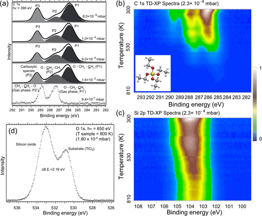
Figure 9. APXPS investigation of adsorption of TEOS on TiO2(110) and SiO2 CVD. (a) C 1s APXP spectra at the indicated pressures recorded during room temperature adsorption. The bottom spectrum is the gas phase spectrum of TEOS. (b) C 1s and (c) Si 2p APXP spectra measured during heating of the TiO2(110) sample in a TEOS atmosphere at 2.3 × 10⁻⁴ mbar pressure. (d) O 1s spectrum recorded at the end of the temperature run. Reprinted with permission from [Chaudhary S, Head A R, Sánchez-de-Armas R, Tissot H, Olivieri G,Bournel F, Montelius L, Ye L, Rochet F, Gallet J J, Brena B and Schnadt J 2015 J. Phys. Chem. C 119 19149]. Copyright (2015) American Chemical Society.
Download figure:
Standard image High-resolution imageIn the following we present results from a few CVD and ALD APXPS studies in order to highlight some of the information content of the experiments and some of the possibilities for obtaining new information on the surface chemistries of CVD and ALD.
5.1. Chemical vapour deposition
Figure 9 shows data from an APXPS study of the adsorption and reaction of tetraethyl orthosilicate (TEOS, (CH3CH2O)4Si, cf inset in figure 9(b)) on a rutile TiO2(110) surface (Chaudhary et al 2015). TEOS has been used for a long time as precursor for SiO2 CVD (Oroshnik and Kraitchman 1968, Rauscher 2001). The SiO2/TiO2 materials combination is of interest in a wide range of applications, including in particular photocatalysis (Chen et al 2015), but also e.g. anti-fouling agents in membranes (Jhaveri and Murthy 2016) and superhydrophilic materials (Houmard et al 2008).
Panel (a) of figure 9 shows the C 1s line measured on the room-temperature TiO2 surface at TEOS pressures from 8 × 10⁻⁹ mbar up to 1.6 × 10⁻⁶ mbar and, in addition, the C 1s spectrum of the TEOS gas phase. The latter exhibits the expected two-component shape with the lower-binding energy peak attributed to the terminal methyl groups and the higher-energy one to –CH2–. The three-peak structure of the surface spectra provides evidence for a surface reaction of TEOS. As before, we attribute the two lower-energy peaks to –CH3 and –CH2–, while the high binding-energy component is attributed to formation of a carboxylate moiety upon dissociation of either Si–O or O–C bonds, resulting in the presence of ethoxy and ethyl groups on the TiO2(110) surface (Chaudhary et al 2015).
The same components are seen in the initial C 1s spectra recorded during a heating run in the presence of 2.3 × 10⁻⁴ mbar TEOS. The data are shown as an image plot in figure 9(b), with the corresponding Si 2p data displayed in figure 9(c). The growth of an SiO2 O 1s signal (figure 9(d)) shows that the heating puts the system into CVD mode. What is interesting now is that APXPS enables one to precisely follow the evolution of the different surface species: The C 1s image plot in figure 9(b) shows that the carboxylate disappears at significantly lower temperature than the other components. This is accompanied by an equalisation of the intensities of the –CH3 and –CH2–. We can conclude that the ethoxy species are considerably more weakly bonded than the ethyl species (cf Chaudhary et al (2015)). Furthermore—and more importantly for the CVD—we can easily and directly identify the temperature needed for a clean CVD process: at 800 K the last remainders of the C 1s lines at a binding energy of 285 eV disappear, and hence this is the preferred temperature for CVD.
The study also provides a good example of the importance of measuring separate gas phase data: in figure 9(a) the energies of the surface and gas phase lines are seen to lie in exactly the same range. For APXP spectra measured at around 10−1 mbar or higher, i.e. when the gas phase signal is sizeable, a separation of the two spectra contributions would be very difficult without further information on the shape and approximate position of the vapour lines.
5.2. Atomic layer deposition
As already described above, ALD is a deposition method that relies on the cyclic exposure of a solid support to two (or possibly more) precursors in the vapour phase (see e.g. Miikkulainen et al (2013)). In order to achieve a highly controlled deposition the adsorption and reaction of the precursor with the surface needs to be self-limited. ALD has been used to deposit a wide range of materials, but prototypical is the deposition of oxides such as Al2O3, SiO2, HfO2 and TiO2. In the oxide ALD processes the surface is exposed to a metal precursor in the first half-cycle of the reaction and then to an oxygen source such as molecular oxygen, water, ozone or oxygen plasma in the second half cycle. In the full cycle a submonolayer up to a full monolayer of oxide is deposited, although typical growth patterns entail deposition of considerably less than a monolayer of material within one cycle. The process is then repeated until the desired film thickness is reached.
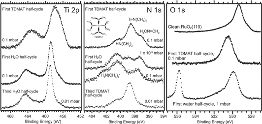
Figure 10. APXPS study of TiO2 ALD from TDMAT and H2O on RuO2(110): Ti 2p, N 1s and O 1s APXP spectra acquired during the initial cycles of ALD. The sample temperature was 110 °C, and a photon energy of 580 eV was used in the recording of all spectra. Reprinted with permission from [Head A R, Chaudhary S, Olivieri G, Bournel F, Andersen J N, Rochet F, Gallet J J and Schnadt J 2016a J. Phys. Chem. C 120 243]. Copyright (2016) American Chemical Society.
Download figure:
Standard image High-resolution image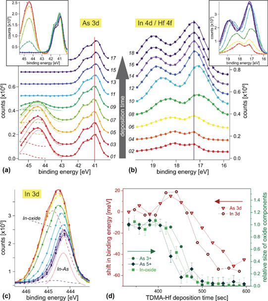
Figure 11. APXPS study of the initial half-cycle of HfO2 ALD on InAs(100) from TDMAHf. (a) Time-resolved As 3d APXP spectra, (b) corresponding In 4d/Hf 4f APXP spectra, (c) In 3d APXP spectra and (d) analysis of the time evolution of the different spectral components. The data were recorded at a sample temperature of 220 °C and a TDMAHf pressure of 8 × 10⁻³ mbar. The photon energy used in recording the spectra in (a) and (b) 330 eV and 570 eV for those in (b) and (d). Reproduced from [Timm R, Head A R, Yngman S, Knutsson J V, Hjort M, McKibbin S R, Troian A, Persson O, Urpelainen S, Knudsen J, Schnadt J and Mikkelsen A 2018 Nat. Commun. 9 1412]. CC BY 4.0.
Download figure:
Standard image High-resolution image
For most ALD processes the underlying ALD chemistry remains largely unexplored beyond idealised reaction mechanism based on general chemistry principles. For thermal ALD processes based on an alkylamido metal precursor such as tetrakis(dimethylamido) titanium (TDMAT) and water the proposed reaction mechanism is that of ligand exchange (Xie et al 2007):
Metal half-cycle:
Ti(N(CH3)2)4 + surface–OH → NH(CH3)2 + surface–O–Ti(N(CH3)2)3.
Oxygen half-cycle:
Surface–O–Ti(N(CH3)2)3 + 2H2O → surface–TiO2–OH + 3NH(CH3)2.
Hence, the proposed reaction mechanism requires surface-terminating hydroxyls for the reaction to proceed and it stipulates the presence of amido ligands as the only non-metal oxide species on the surface after the metal half-cycle. Furthermore, it stipulates that Ti only occurs in its +4 oxidation state. Consideration of the APXPS data acquired before and during the initial metal half-cycle of TiO2 ALD on RuO2(110) from TDMAT and water in figure 10(a) provides a quite different picture (Head et al 2016): no hydroxyl peak is discernible in the O 1s spectrum of the clean RuO2(110) surface; it is free from hydroxyls. During the first TDMAT half-cycle the Ti 2p lineshape provides evidence for the presence of the +2, +3 and +4 oxidation states of Ti. The corresponding N 1s data clearly show that the dominating amido surface ligands are accompanied by other surface species, which we identify as dimethylamine and methyl methylene imine.
In the subsequent oxygen half-cycle the amido surface ligands react with the water, while the dimethylammonium and methyl methylene imine adsorbates persist. The reaction is initiated at low pressure, but only after raising the pressure to 0.1 mbar this reaction is completed. Furthermore, it is accompanied by another reaction, namely the formation of dimethylammonium ions.
Clearly, the surface chemistry of the initial ALD process is quite different from the stipulated one. In the initial metal half-cycle ALD proceeds without hydroxyl reaction partners. The reaction mechanism is likely dominated by a β-hydride elimination reaction, resulting in the formation of methyl methylene imine, dimethylamine and a surface Ti complex in which one (or more) of the amido ligands has been replaced by the RuO2(110) surface. First in subsequent ALD cycles a ligand exchange reaction mechanism seems to take over, as is seen from the absence of an imine peak in the N 1s spectrum recorded during the third TDMAT half-cycle and the formation of a hydroxyl peak in the O 1s spectrum during the first water half-cycle.
The APXP spectra of the TiO2 ALD study were recorded in situ and thus during the ongoing ALD, but without any further time resolution. The addition of a time dimension can provide very valuable, additional information of the surface chemistry of the ALD process. This is illustrated for the initial metal half-cycle of HfO2 ALD on a native oxide-covered InAs(100) wafer, cf figure 11 (Timm et al 2018). As metal precursor tetrakis(dimethylamido) hafnium (TDMAHf) was used; the standardly proposed reaction mechanism is the same as for the TDMAT precursor shown above, i.e. the reaction is thought to proceed via ligand exchange. Here, the focus is, however, on the self-cleaning process of the InAs(100) surface (i.e. the native oxide removal) rather than the reaction mechanism.
During the initial Hf half-cycle the evolution of the intensities of the As 3d line, with the native oxide on the InAs(100) surface giving rise to the peak at 44.5 eV binding energy and the InAs bulk peak at 41 eV, the overlapping In 4d and Hf 4f peaks and the In 3d peak, with the oxide component at around 445 eV and the bulk component at 444.2 eV, was followed (figures 11(a)–(c)). The time required to record a single spectrum was on the order of 10 s. The As 3d and In 4d/Hf 4f spectra in figures 11(a) and (b) were recorded alternately, resulting in a time resolution of approximately 20 s. Correspondingly, the spectra in figure 1(c) and the As 3d spectra underlying the data in figure 11(d) were also recorded alternately.
In the As 3d and In 3d APXP spectra the disappearance of the oxide peak due to the interaction of the surface with the TDMAHf precursor can easily be followed in real time. A more detailed analysis of the As 3d lineshape (Timm et al 2018) then shows that the As +5 oxide component (as in As2O5 or InAsO4) disappears before the In oxide and the As +3 oxide (as in As2O3) components (figure 11(d)). Since AsO3 is less stable than As2O5 or InAsO4 the finding is counter-intuitive at first sight. The native oxide removal does not seem to be controlled by thermodynamics, but rather by the bonding geometries of the oxygen atoms in the oxide: that of the oxygen atoms in As2O5 seem to provide a better interaction site for the TDMAHf precursor.
Notable is also the low binding energy of the Hf 4f signal in the initial stage of interaction (figure 11(b)), green and light blue spectra), which is superseded by a considerably higher binding energy at somewhat later stages. We interpret this finding as evidence for a two-step reaction during TMDAHf adsorption: initially, TDMAHf is adsorbed molecularly, and dissociation and Hf–O bond formation occurs first during the second reaction step. The unexpectedly low Hf 4f binding energy of the molecularly adsorbed precursor can be explained in a reaction mechanism that foresees a nucleophilic attack by the N lone pair of one of the dimethylamido ligands on surface As or In atoms. The attack lowers the electron density on the N atom, but increases it on the adjacent Hf atoms, and, hence, a lower Hf 4f binding energy is observed.
The time resolution of the APXPS data provides insight into chemical information that without time resolution would have gone unnoticed. In particular, it opens a door towards a precise understanding of reaction mechanisms, here of the surface chemistry of the initial ALD. This surface chemistry may have decisive influence on the structure and quality of the deposited film. Learning to understand the chemistry results in entirely new possibilities for tailoring the chemistry and, in a longer-term improve the quality of ALD processes and of the thin films deposited by ALD.
The time resolution in the above example was still quite limited with a frame rate of around 0.1 Hz. For many systems the high photon fluxes at third or fourth generation synchrotron radiation sources allows for considerably higher frame rates, not only with delay-line detectors, but also with modern MCP/CCD detectors that can operate with frame rates of 100 Hz or more. This also implies that APXPS enters the age of big—or at least bigger—data, and the detailed analysis of APXP spectra is becoming a formidable challenge, which requires a hitherto largely unseen advanced computational expertise of APXPS users.
6. Conclusions
APXPS is an experimental method that in a few years' time will see its half-centennial birthday. During the first half of its hitherto life-span APXPS was a laboratory-based technique, and only a handful of instruments existed. The advent of third-generation synchrotron light sources, coupled with the development of differentially pumped electron lens systems for electron energy analysers, made possible the breakthrough of the method in the early 2000s. Now, twenty years later, APXPS is a mature and well-established experimental technique for catalysis, surface science, materials science and other fields. The APXPS research area's maturity notwithstanding, the community remains highly vibrant and on the constant outlook for instrumental improvement and new areas of application of APXPS. It is rather fascinating to see that the development of APXPS as a synchrotron-based technique now has led to a fantastic upswing of APXPS laboratory activities. The conditions of synchrotron and laboratory activities are very different, which implies that synchrotron and laboratory have to be used in different, but complementing ways. Where the photon flux of synchrotron instruments allows intensity-hungry experiments with e.g. time or spatial resolution, laboratory experiments provide space for more risky experiments that cannot be fit into a single week or less of beamtime and for experiments that map large parameter spaces. Many frontiers exist in APXPS research. Some of them we have identified in this topical review, and these are the challenge of studying surface chemical reactions that are complex in terms of sample structure and/or chemistry; the challenge of higher and even more realistic pressures than what most of present APXPS setups allow—the 1 bar limit has been passed by now, but there is plenty of room for exciting epxeriments between the present standard of around 1 mbar and atmospheric pressure; the challenge of electrochemistry and flow cells, propelling APXPS even more into the heart of energy materials research, so urgently needed if we would like to solve the environmental challenges that mankind faces; the challenge of time-resolved and pump-probe studies, which also bring along the challenge of big data; the challenge of meaningfully combining APXPS with other spectroscopy and microscopy methods that probe exactly the same sample as APXPS at the same moment in time; and the challenge of increasing the information depth of APXPS by obtaining structural and spatial information, e.g. from photoelectron diffraction, photoelectron microscopy and SWAPPS. We are looking forward to new exciting developments in APXPS research!
Acknowledgments
We gratefully acknowledge all of our colleagues who took part in the conception, measurement, analysis and publication of the data presented in this topical review and the beamline staff at the TEMPO beamline at SOLEIL and the SPECIES and HIPPIE beamlines at the MAX IV Laboratory for their support during beamtimes (in alphabetical order): Jesper N Andersen, Margit Andersson, Virgínia Boix, Barbara Brena, Fabrice Bournel, Filippo Cavalca, Shilpi Chaudhary, Lenart Dudy, Jean-Jacques Gallet, Tamires Gallo, Ashley R Head, Martin Hjort, Johan V Knutsson, Sarah McKibbin, Esko Kokkonen, Anders Mikkelsen, Mikko-Heikki Mikkelä, Lars Montelius, Giorgia Olivieri, Olof Persson, François Rochet, Rocío Sánchez-de-Armas, Mattia Scardamaglia, Andrey Shavorskiy, Rainer Timm, Héloïse Tissot, Andrea Troian, Lei Ye, Samuli Urpelainen, Sofie Yngman, Suyun Zhu.
The assistance of Axel Knop-Gericke, Hendrik Bluhm, John Åhlund (Scienta Omicron) and Liana Socaciu-Siebert (SPECS) in putting together the data in figure 2 is gratefully acknowledged.
Vetenskapsrådet (Swedish Research Council, Grant Nos. 2010-5080, 2011-4241, 2012-05815, 2012-03850, 2017-03871, 2017-04108, 2017-04840) and the European Commission through the Marie Skłodowska Curie Initial Training Network SMALL (Grant No. MCITN-238804) are acknowledged for funding.