
Abstract
The identification of the stable phases in alloy materials is challenging because composition affects the structural stability of different intermediate phases. Computational simulation, via multiscale modelling approaches, can significantly accelerate the exploration of phase space and help to identify stable phases. Here, we apply such new approaches to understand the complex phase diagram of binary alloys of PdZn, with the relative stability of structural polymorphs considered through application of density functional theory coupled with cluster expansion (CE). The experimental phase diagram has several competing crystal structures, and we focus on three different closed-packed phases that are commonly observed for PdZn, namely the face-centred cubic (FCC), body-centred tetragonal (BCT) and hexagonal close packed (HCP), to identify their respective stability ranges. Our multiscale approach confirms a narrow range of stability for the BCT mixed alloy, within the Zn concentration range from 43.75% to 50%, which aligns with experimental observations. We subsequently use CE to show that the phases are competitive across all concentrations, but with the FCC alloy phase favoured for Zn concentrations below 43.75%, and that the HCP structure favoured for Zn-rich concentrations. Our methodology and results provide a platform for future investigations of PdZn and other close-packed alloy systems with multiscale modelling techniques.
Export citation and abstract BibTeX RIS

Original content from this work may be used under the terms of the Creative Commons Attribution 4.0 license. Any further distribution of this work must maintain attribution to the author(s) and the title of the work, journal citation and DOI.
1. Introduction
Computational approaches now provide opportunities for accelerated exploration of material phase space, though significant challenges remain [1–3]. Whilst experimental verification of relative phase stability is challenging, the ability to interrogate and understand phase diagrams through application of computational modelling can be achieved by taking initial estimates of the thermodynamically accessible phases, and their boundaries, and interpolating between the available data points and extrapolating to experimentally inaccessible regions. Computational explorations of phase diagrams typically combine high throughput first-principles calculations and data mining techniques, and are facilitated by the availability of extensive thermodynamic databases [4, 5]. These modern capabilities allow the prediction of new stable materials, and their properties, and understanding of phase stability for compositions that have not been previously considered experimentally.
In catalysis, the stability of a specific phase can alter reaction efficacy. The PdZn alloy is widely studied owing to its catalytic performance toward CO2 hydrogenation and related catalytic chemistry. Compared to Cu based catalysts, Pd/ZnO has greater stability for the methanol steam reforming reaction [6]. Pd/ZnO catalysts can be active for CO2 hydrogenation to methanol depending on the choice of preparation method and the Pd precursor, which affects the selectivity of the products. Pd has a strong tendency to form intermetallic species with ZnO when exposed at a high temperature under a reducing environment, such as during hydrogenation reactions [7]. For the CO2 hydrogenation reaction, the proximity between the metal and substrate stabilises the formate (HCOO) species, which is reported as the intermediate on PdZn alloy.
The complex phase diagram of PdZn [8] comprises several structures, as shown in figure 1. Amongst the different phases, the most important are:
- (1)The body-centred tetragonal (BCT) structure named β-PdZn, in the P4/mmm space group, which is observed at compositions close to 1:1 at the material's surface for temperatures of 230 °C, but does not penetrate to the bulk until 500 °C [9].
- (2)The face-centred cubic (FCC) phase with random substitutional alloying, denoted α-PdZn, which is observed in the Pd-rich region of the PdZn phase diagram [9], influenced by the stability of the Pd FCC structure.
- (3)The intermediate phases that include Pd2Zn, Pd2Zn3, PdZn2, Pd2Zn9 [10]. Pd2Zn is especially interesting as it lies in the area between the α- and β-PdZn. An intermediate Pd2Zn phase was observed to form at intermediate temperatures during the increase from room temperature to 600 °C [11]. Moreover, in a recent paper, Wang et al have identified different intermetallics [12] such as Pd2Zn3, PdZn2 and Pd3Zn10 during the synthesis of AgPd30/CuNi18Zn26 bilayer laminated composites.
- (4)The preferred phases of the individual elements, which dominate at the borders of the phase diagram: FCC is observed at high Pd concentrations (from 70% to 100%) while the hexagonal close packed (HCP) phase is present at high Zn concentrations (from 85% to 100%).

Figure 1. Experimental phase diagram taken from [10] 2013, reprinted by permission of the publisher (Taylor & Francis Ltd, www.tandfonline.com). The white regions represent the unstable compositions that decompose into stable compositions, which are represented by the grey regions. The abbreviations of rt and ht are for room and high temperature, respectively, and L for liquid. The data points given indicate the temperatures reported. Symbols depict important data from: □ [13, 14], ○ [15], △ [16], ◊ [17, 18],▽ [19], • [20], and ▲ [8, 21, 22].
Download figure:
Standard image High-resolution imageInformation on the relative stability of competing structural phases as a function of composition can help to drive forward materials design and application, especially in fields such as heterogeneous catalysis where alloyed metals play a crucial role. However, developing knowledge of multi-element phase diagrams remains a significant challenge, due to the combinatorial problem of atomic distribution. Several approaches have been developed to address this challenge, such as global optimisation and parameterised models for accelerated sampling. Cluster expansion (CE) is a parametric approach that has been widely and successfully used for alloys [23] as configuration-dependent properties (such as energy) can be described by the CE model once trained appropriately. Energy is a key property of interest when determining phase stability, and can be obtained from e.g. first-principles calculations; for semiconductor materials, CE trained with bandgap data [24] has been employed alternatively.
In this article, we extend previous efforts to model alloy phase diagrams by investigating the complex PdZn landscape with a combination of density functional theory (DFT) and CE techniques. We aim to develop models of the bulk phases that can subsequently be used to predict properties and to explore surface structures and properties. We also aim to demonstrate the potential capability of coupling first-principles modelling with parameterised models for accelerated exploration of complex materials phase space. Our methodology and results are presented herein, followed by a conclusion discussing current opportunities and challenges.
2. Methodology
2.1. Density functional theory
DFT calculations have been performed with the Fritz Haber Institute ab initio materials simulations (FHI-aims) all-electron full-potential software package (date stamp: 210311) [25] coupled with the LibXC library [26]. Unless stated, all calculations were performed using the mBEEF exchange-correlation functional, a 'light' basis set (version 2010), and a Monkhorst-Pack k-grid sampling density of one k-point per 0.018 × 2π Å−1, as determined as optimal in previous studies for Pd, Cu and Zn monometallic materials [27]. The self-consistent field cycle was deemed converged when the changes in the total energy and electron density were less than 1 × 10⁻⁶ eV and 1 × 10⁻⁶ e a0 3, respectively. Throughout, a spin-paired configuration has been used with scalar relativity included via the atomic zero order regular approximation [28]. The unit cell optimisation was performed using the analytical stress tensor in FHI-aims. Unit cell and geometry optimisations were applied until forces on all unconstrained atoms and lattice vectors were less than 0.05 eV Å−1. To demonstrate validity of our force convergence criterion, a more stringent 0.01 eV Å−1 force convergence criterion was tested on the ordered PdZn structure, and the difference in energy was less than 0.0001 eV/atom without any structural changes.
2.2. Cluster expansion
The configurational space of a binary system with composition A1−x
Bx
, when represented with a supercell containing N lattice sites, gives rise to 2N
configurations without considering symmetries, thus yielding a combinatorial explosion of the number of configurations with supercell size. The quantity of configurations poses a challenge to ab initio descriptions of alloy phase diagrams, due to the computational expense in performing simulations. CE provides capability to address this challenge, offering a compact and numerically efficient way to describe the configurational dependence of physical properties for mixed systems [29] while retaining ab initio accuracy. In CE, the occupation of every crystal site is represented by a variable  , which takes the value (+1) if the site is occupied by atom A or (−1) if the site is occupied by atom B. A configuration of the
  -site lattice can be represented as σ = (
 ,
,  ,...,
,...,  ). Then, the energy E(σ) is modelled by [30]:
Here, the summation runs over  symmetrically inequivalent sets of crystal sites, termed clusters
  .
.  is the effective cluster interaction (ECI) for cluster
  ,
,  is the corresponding cluster multiplicity, and
  is the cluster correlation defined as
The overline represents the average over all  clusters symmetrically equivalent to
  . Although the number of clusters is in principle infinite, for practical applications one must truncate the summation, resulting in a finite set of clusters of size
  . A few examples of the kind of Zn clusters contained in the clusters set for the PdZn alloy starting from a pristine Pd supercell are shown in figure 2.
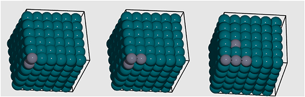
Figure 2. Examples of 2-, 3- and 4-body clusters generated for PdZn starting from a pristine Pd supercell. Pd is presented by blue spheres and Zn by grey spheres. The black lines represent the supercell boundaries.
Download figure:
Standard image High-resolution imageIn this work, CE models have been built using the CELL package [31], a python package for CE with a focus on complex alloys. In CELL, the ECIs are obtained by fitting the model of equation (1) to a set of  ab initio calculations for configurations
  :
:
Here,  ,
,  with
with  the property computed ab initio for structure
  ;
;  is the corresponding CE predictions using the model of equation (1), computed as
  , with
  the matrix of cluster correlations
  ; and
; and  and
and  are the regularisation parameter and the regularisation function, respectively, whose role in building CE models are explained below.
In this work, we build CE models of the energy of mixing for each of the three crystallographic representations of the phase diagram: FCC, BCT and HCP. The energy of mixing per atom is given by:
where Etot is the calculated total DFT energy for the relaxed structure; EPd and EZn are the energy of the respective pure Pd and Zn bulk structures in the same phase, n is the total number of atoms in the structure, and xZn is the number of Zn atoms.
The formation energy per atom, Efor, is calculated taking in account the most stable phases of Pd and Zn, which are FCC and HCP, respectively. Therefore, for the alloys in an FCC configuration Efor is calculated as:
and for an HCP configuration as:
where  is the mixing energy per atom calculated in equation (4);
  is the Zn concentration;
  is the chemical potential difference for Zn in the non-ground state (GS) FCC structure, defined as
  0.036 eV/atom; and
  is a similar quantity calculated for Pd in the non-GS HCP structure, defined as
  = 0.026 eV/atom.
For training of the CE models, supercells consisting of 16 atoms were considered, which is sufficient to reproduce many possible configurations for each substitution, while being still tractable by ab initio calculations within a reasonable computing time.
Once the training data are obtained, consisting of the supercell structures and the corresponding Emix computed via ab initio approaches, the remaining task is to find the optimal CE model, which entails determining (i) the optimal set of clusters and (ii) the ECIs yielding the best possible predictions. For (i) we have considered strategies of subset selection, combinatorial search, and least absolute shrinkage and selection operator (LASSO) [32]. All of them are aimed at yielding sparse models, i.e. models with few clusters that avoid over fitting and minimise test errors. They are explained in more detail in section 4.1.4. For (ii) we have used linear regression and ridge regression, which correspond to taking  and
and  in equation (3), respectively [32].
2.3. Metropolis Monte Carlo
The Metropolis Monte-Carlo (MMC) approach [33] is implemented in the CELL package and allows simulations in the canonical ensemble at constant pressure and temperature. During MMC, new configurations are generated by swapping two random atoms in the previous structure. Each of the new structures, with energy E1, are accepted with the probability:
where E0 is the energy of the structure before the swap, T is the given simulation temperature, and kB is the Boltzmann constant.
The specific heat capacity, Cp , is calculated as:
where  and
and  are the ensemble-averaged energy and the ensemble-averaged squared energy at T, respectively.
3. Atomistic model optimisation
3.1. FCC
A dataset has been built consisting of derivative structures from a  supercell of Pd (16 atoms). The FCC parent lattice and an example derivative structure are shown in figure 3. The primitive cell for Pd has an optimised lattice parameter of
  Å, which corresponds to supercell parameters of
  Å and
Å and  Å, as shown in figure 3. Compositions have been generated with random configurations ranging from 0%–100% concentration of Zn, to obtain data for the full composition range.
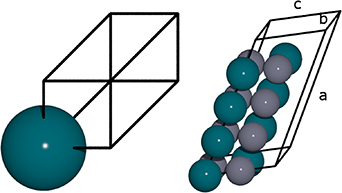
Figure 3. Left: representation of the parent primitive FCC lattice; Right:  supercell. Blue (grey) spheres represent Pd (Zn) atoms. The supercell lattice vectors are labelled a, b and c.
Download figure:
Standard image High-resolution imageInitially, 100 structures were generated and optimised (unit cell and geometry) using DFT for training the CE model. Then, MMC simulations were performed with the CE model at a temperature of 500 K, with various concentrations, to find new low energy configurations. The final dataset is the combination of the 100 structures generated randomly with the lowest energy structures collected from the MMC simulations. The same approach was taken for primitive  (16 atoms) and for conventional
  (32 atoms) supercells. The lowest energy structures for each concentration tested in the MMC simulations were further optimised; most structures were stable, though a few select systems deviated significantly from the ideal FCC parameters, namely
  and
and  as shown in figure 4. The factor of 2 in
  accounts for the asymmetry in the
  supercell expansion of the unit cell.
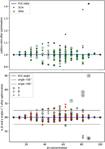
Figure 4. Variation of the lattice parameter ratios (top) and unit cell angles (bottom) after structure optimisation for FCC primitive models. A key is provided in both graphs, with grey circles in the lower graph highlighting the structures with high angular distortion. The horizontal black dashed lines indicate a threshold ±5 °, which is applied when considering filtering of the dataset (section 4).
Download figure:
Standard image High-resolution imageDistorted structures with large  ratios have large deviations in cell angles too. Some structures that present very large distortions are obtained for Zn-rich cases [62.5, 81.25 and 87.5%, represented by the grey circles in figure 4 (bottom)] and could be related to structures relaxing toward orthorhombic phases such as the PdZn2 and Pd2Zn9 intermetallic alloys, which are stable for these compositions [13]. Examples of the distorted structures are given in figure 5: a structure with an 87.5% concentration of Zn is presented, which optimised to a triclinic phase (α = 44.96°, β = 44.68° and γ = 59.94°).
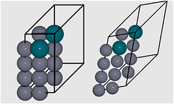
Figure 5. Left: an initial FCC primitive  structure; Right: the same structure after geometry optimisation, showing cell distortion.
Download figure:
Standard image High-resolution imageAn additional 82 FCC configurations were identified during the MMC stages. There were collated with the original 100 structures to form a training dataset of 182 structures.
3.2. BCT
For a concentration of 50% Zn, PdZn forms a stable tetragonal  structure, denoted the
  -phase [9]. The
  structure can be viewed either as (i) a BCT-based superstructure with a stacking of pure Pd and Zn layers, or as (ii) a tetragonal distortion of an FCC-based superstructure. The experimental
  ratio is 1.15 when the BCT representation (i) is used, which contrasts distinctly with a
  ratio of 1.41 for the ideal FCC structure. Given the importance of the
  structure for the PdZn alloy, a dataset of derivative structures was generated from BCT-based supercells with an initial
  ratio of 1.15. The experimental
  -phase, which is depicted in figure 6, is included in this set. The computed lattice parameters are a =b =2.87 Å and c =3.36 Å, which corresponds to
  = 1.17, in close agreement with experiment [34].
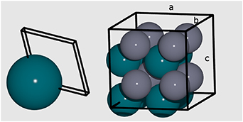
Figure 6. Parent lattice used for the BCT model (left) and conventional supercell (right); Pd represented by blue spheres and Zn by grey spheres, with unit cell vectors labelled as a, b, and c.
Download figure:
Standard image High-resolution imageBased on the conventional supercell in figure 6, 100 random structures were generated with Zn concentrations ranging from 0% to 100%, in a similar approach to the initial FCC dataset creation. The calculated  and
and  ratios, and the cell angles α, β, and γ, are given in figure 7 for the optimised structures.
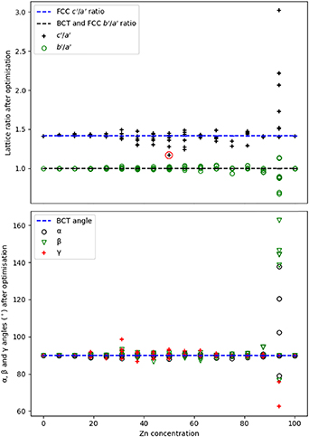
Figure 7. Lattice parameters (top) and angles (bottom) after the atomistic optimisation for the BCT conventional supercell with varying Zn concentration. A key is provided on each graph; the red circle on the lattice parameter plot highlights the lowest energy structure, corresponding to  = 1.17.
Download figure:
Standard image High-resolution imageStructural optimisation of the BCT models resulted in 92% conversion to a  ratio of 1.39–1.41, while
  remained as unity, indicating that most structures converted to an FCC phase. The conversion observed is unsurprising given the narrow range of stability for the
  structure in experiment; furthermore, the conversion of structures with high Pd concentrations (>70%) to FCC agrees with experimental findings that this phase is dominant in Pd-rich compositions. For the Zn concentration of 50%, the
  ratio is recorded as ranging from 1.17 to around 1.41, with 29% of structures having
  ratios below 1.30. The lowest-energy structure, corresponding to a
  ratio of 1.17 in the
  -phase, is marked with a red circle in figure 7 (top), while all the others have higher
  ratios and could correspond to metastable phases of PdZn. A
  ratio of 1.29 and 1.30 is also observed for some structures with Zn concentrations between
  and
and  , with the
  ratio remaining close to unity. Thus, these structures could be considered as BCT phases because they have not fully converted to an FCC structure. It is noted that the changes in
  with varying Zn concentration are less pronounced than for
  , except for the Zn concentration of 93.75% where large distortions in all ratios were accompanied by significant angular distortions.
Overall, no consistent BCT-based training set could be derived for building a CE model, as very few structures remained in a BCT phase after geometry optimisation. Nonetheless, our calculations confirm experimental observations regarding (i) the stability of the  -phase, (ii) the narrow stability range around 50% Zn concentration for this phase and (iii) the general stability of the FCC phase for low Zn concentrations.
3.3. HCP
Analogous to the procedure used for generating the FCC and BCT structures that formed the CE datasets, 100 random structures with an HCP primitive  supercell structure, containing 16 atoms, were generated with Zn concentrations ranging from 0% to 100%; further structures were added via a MMC configuration search at 500 K. The optimised lattice parameters for the Pd 2-atom primitive cell (figure 8) are a'' = b'' = 5.41 Å and c'' = 8.90 Å. An example of the supercell model employed to generate the derivative structures is also provided in figure 8.
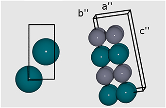
Figure 8. Left: Parent primitive cell used for the HCP model; Right: supercell of the same HCP model. The Pd and Zn atoms are represented by blue and grey spheres, respectively. The unit cell boundaries are defined by a black line, with labels indicating the lattice vectors.
Download figure:
Standard image High-resolution imageThe structural results from optimising the HCP models, specifically the  ratio and the cell angles, are presented in figure 9. The lattice parameter ratio (
 ) varies from 0.94 to 1.04 except for two structures with ratios >1.05, as highlighted by the red circles in figure 9 (top). These two structures are for Zn concentrations of 31.25% and 62.5%. These compositions are close to those of the orthorhombic Pd2Zn and PdZn2 structures in the phase diagram [10], and therefore we believe these structures were relaxing to the orthorhombic phase. The unit cell angles were less distorted than the lattice parameters for the HCP structures overall; γ distorts by less than 4° in most structures, while α distorts by a maximum of 9°, which is observed for Zn concentrations of 75%, 37.5% and 57% (figure 9, bottom).
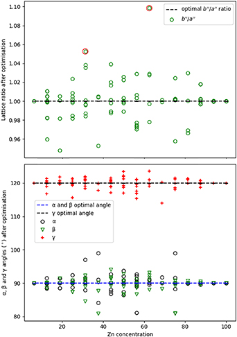
Figure 9. Ratio of lattice parameters  for the HCP models (top) and optimised cell angles (bottom) after the atomistic optimisation for the HCP supercell with varying Zn concentration. Red circles in the top graph highlight the orthorhombic Pd2Zn and PdZn2 structures.
Download figure:
Standard image High-resolution image4. CE model optimisation
The generation and optimisation of the CE models for FCC and HCP systems are discussed herein. The description of the different estimators used in the CE model for building and optimisation tasks are also provided.
4.1. FCC
4.1.1. Effect of distortion.
As discussed in section 3.1, structure optimisation of the FCC model leads to various degrees of distortions in the structures contained in the datasets. Here, we investigate how the presence of strongly distorted structures in a dataset can affect the quality of the obtained CE models. To this end, different thresholds are tested for the permissible angles between unit cell vectors when creating the training dataset. Structures that lie outside the threshold after relaxation are excluded from the dataset, with the final dataset tested for training of the FCC CE model. Three different filters were applied based on angular distortion, namely:
- (1)All optimised structures are included (i.e. no filter is applied).
- (2)Only structures with angles that deviate by less than ±10° from the ideal FCC angle, i.e. 50° ⩽ α, β, γ ⩽ 60°, were included. 96.64% of structures from the initial training set comply with this filter.
- (3)Only structures with angles that deviate by less than ±5° from the ideal FCC angles, i.e. 55° ⩽ α, β, γ ⩽ 65°, are included. 89% of structures from the initial training set comply with this filter.
In table 1, the errors estimated by cross-validation (CV) [32] using the LASSO selector are presented when applying each threshold. CV tests the model's ability to predict new data that was not used in its creation and allows the identification of over- or under-fitting, as well as giving an insight as to how the model will generalise to an independent or new dataset.
Table 1. Errors in eV/atom for cross-validation (CV) when selection rules were applied using the LASSO selector. The root mean squared error (RMSE), the mean absolute errors (MAEs), and the maximum absolute errors (MaxAE) are reported from the CV testing.
| Filter 1 (No filter) | Filter 2 (±10°) | Filter 3 (±5°) | |
|---|---|---|---|
| RMSE (eV/atom) | 0.014 98 | 0.008 10 | 0.005 92 |
| MAE (eV/atom) | 0.011 61 | 0.006 11 | 0.004 39 |
| MaxAE (eV/atom) | 0.039 90 | 0.028 34 | 0.018 14 |
Introduction of filters for the structures that are included in the training dataset has a notable impact on the CV results. Table 1 shows an improvement of 65%, 62% and 55% for the RMSE, MAE and MaxAE, respectively, has been obtained with the CE model trained on a dataset where threshold (3) was applied; a similar but smaller improvement occurs when applying threshold (2), i.e. including structures with angular deviation in the unit cell ⩽10°, with improvements of 45%, 47% and 29% for the RMSE, MAE and MaxAE, respectively. The results highlight the importance of excluding structures from the training set that significantly distort from the initial FCC geometry. The improvement is noted as not simply due to reduction of the dataset size when the threshold is applied, as will be discussed in the next subsection. We conclude that a filter of ±5° on the unit cell angles is necessary to create a high-quality CE model with low test error. To visualise the data that is removed from the training set with this criterion, two horizontal dashed lines are given in figure 4 (bottom) that indicate the threshold boundaries; all data outside those boundaries are discarded from the dataset for model training.
4.1.2. Dataset size.
Different dataset sizes, with 50, 100 and 182 structures, were considered when constructing the CE model. The same settings were applied as in section 4.1.1, with LASSO as the selector and the ridge regression estimator with  1.0 × 10⁻⁶. The absolute errors (AE) for CV with the different datasets are reported in figure 10.

Figure 10. Plot of dataset size against AE for the CE models constructed with datasets containing 50, 100 and 182 structures. The median AE is indicated by the horizontal orange line and represents 50% of the data; the lower edge of each box represents the boundary for the lower 25% of the data (Q1) and the upper 75% of the data (Q3). The lower whisker corresponds to the lowest value observed, while the higher whisker corresponds to the largest value obtained that is deemed accurate. Circles indicate outliers, i.e. data points that are not well captured by the model. The green triangle corresponds to the mean of AE on the given dataset.
Download figure:
Standard image High-resolution imageFor the three CE models, the minimum CV AE is the same (0 eV/atom); however, the average AE average (green triangle in figure 10) is greatest for the model created from the smallest dataset, and smallest for the model with the largest number of structures. The same trend exists for the median of the AE distribution. For the CE model trained on a dataset with 50 structures, three outliers are identified in CV with large AEs of 0.038, 0.028 and 0.019 eV/atom. The outliers have smaller errors for the other CE models: 0.021, 0.019, and 0.016 eV/atom for the CE model trained on a dataset with 100 structures; and 0.019, 0.017, and 0.013 eV/atom for the CE model trained on a dataset with 182 structures.
In conclusion, adding more structures to the training dataset leads to an improvement of the CE model, and validates CE model optimisation with the largest accurate dataset available. The improvement obtained when increasing the dataset size from 100 to 182 structures is small, indicating that our estimation of the test error may be close to the intrinsic error of the dataset [32]. Nevertheless, a numerical benefit is observed from using the largest dataset for CE model training, and herein the FCC CE model is built using all available 182 structures (which all comply with previous filtering criteria).
4.1.3. Clusters pool size.
The quality of the CE model can be affected by the number of clusters,  , referred to herein as the clusters pool size. A larger number of clusters are expected to yield better CE models, as more clusters may lead to better fitting in the cluster selection task, though this comes with a computational overhead that scales unfavourably. In this subsection, the performance of the CE model is reviewed as a function of
  , which allows identification of optimal criteria for determining the cluster pool size. The results of testing are presented in table 2.
Table 2. Breakdown of clusters available when considering specific n-body interactions. For a given number of n-body interactions and a maximum radius on these interactions (first and second row, respectively), the corresponding number of clusters is given (third row). The maximum radius given of 5.5, 7.3, 8.3, and 9.6 Å, correspond to the 3rd, 5th, 6th and 8th Pd bulk neighbour, respectively.
| n-body interactions | 1 | 2 | 3 | 4 | 5 | 6 |
|---|---|---|---|---|---|---|
| Maximum radius (Å) | 0 | 9.6 | 8.3 | 7.3 | 5.5 | 5.5 |
| Available clusters, Ncl,n | 1 | 8 | 29 | 101 | 17 | 16 |
The maximum radius for a given system is the interaction distance, represented by a sphere with given radius, within which substitutions are allowed. For example, when adding a single Zn substitution, there cannot be other Zn interactions and so the maximum radius is 0 Å, as presented in table 2. When including more substitutions, the maximum radius within which a Zn–Zn substitution can occur depends on the size of the supercell; in our case, all possibilities in a  supercell were considered. Taking symmetry and periodicity into account, the maximum radius possible for Zn–Zn pairs is 9.6 Å; however, as the inclusion of more clusters can result in over fitting of the model, the maximum radius for clusters of 3, 4, 5, and 6-body Zn was limited to the 8th, 6th, and 3rd Zn–Zn neighbour distances, respectively.
The number of clusters available increases non-linearly with consideration of larger n-body interactions. When considering both 1- and 2-body clusters,  ; consideration of all clusters up to 3-, 4-, 5-, and 6-body clusters results in
  , 139, 156, and 172, respectively.
CE models were obtained using these varying considerations for the n-body interactions, via application of the limited Ncl . Model fittings was performed using the LASSO selector and ridge as estimator, and the AE in CV is presented in figure 11.
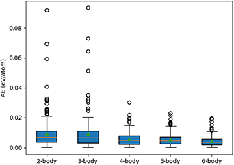
Figure 11. AE errors in eV/atom as a function of Ncl values, considering 1- to 6-body interactions cumulatively. The colour and shape coding are the same as figure 10.
Download figure:
Standard image High-resolution imageIn figure 11, the AE decreases with increasing  . The MAE, indicated with a green triangle, is largest when only up to 3-body clusters are considered in the model definition (0.094 eV/atom). The error reduces by 67%, to 0.030 eV/atom, when including up to 5-body clusters, and improves marginally only after adding the 6-body clusters. The inclusion of 4-body clusters and greater drastically reduces the test error for outliers, when compared to restriction to only 2- and 3-body interactions, as seen from the circles in figure 11. The addition of clusters with a greater number of many-body interactions reduces the error further, but by a lower quantity; from 5- to 6-body, the improvement is only marginal, in both outliers and MAE, indicating convergence (i.e. that the addition of larger clusters, in terms of bodies or radii, will not yield significant improvements). However, the error for the CE model CV does have the narrowest distribution when considering up to 6-body interactions (Ncl
= 172), as shown by the small boxplot, and therefore the initial set of clusters for building the CE models is chosen to contain interactions up to 6-body clusters (Ncl
= 172).
. The MAE, indicated with a green triangle, is largest when only up to 3-body clusters are considered in the model definition (0.094 eV/atom). The error reduces by 67%, to 0.030 eV/atom, when including up to 5-body clusters, and improves marginally only after adding the 6-body clusters. The inclusion of 4-body clusters and greater drastically reduces the test error for outliers, when compared to restriction to only 2- and 3-body interactions, as seen from the circles in figure 11. The addition of clusters with a greater number of many-body interactions reduces the error further, but by a lower quantity; from 5- to 6-body, the improvement is only marginal, in both outliers and MAE, indicating convergence (i.e. that the addition of larger clusters, in terms of bodies or radii, will not yield significant improvements). However, the error for the CE model CV does have the narrowest distribution when considering up to 6-body interactions (Ncl
= 172), as shown by the small boxplot, and therefore the initial set of clusters for building the CE models is chosen to contain interactions up to 6-body clusters (Ncl
= 172).
4.1.4. Selector type.
Table 3 compares the fit and CV errors for CE models obtained with different selectors, using the settings for the dataset size (182 structures) and initial clusters set size (Ncl = 172) as defined in prior sections. The following estimators have been considered in this work:
-
Linear regression aims at minimising the residual sum of squares between the energy calculated by DFT and the predicted energy using the CE model. It is obtained from equation (3) in the manuscript with

-
Ridge regression corresponds to equation (3) with . The regularisation parameter is obtained by CV.


Table 3. Comparison of the RMSE, MAE, and maximum error (MaxAE), all in eV/atom, obtained with different selectors: subset; LASSO; LASSO-on-residual; and combinatorial search.
| RMSE | MAE | MaxAE | ||
|---|---|---|---|---|
| Subset | Fit | 0.004 55 | 0.003 47 | 0.014 72 |
| CV | 0.008 70 | 0.006 52 | 0.045 05 | |
| LASSO | Fit | 0.003 49 | 0.002 68 | 0.013 15 |
| CV | 0.005 64 | 0.004 28 | 0.019 51 | |
| LASSO-on-residual | Fit | 0.005 86 | 0.004 68 | 0.014 63 |
| CV | 0.006 92 | 0.005 44 | 0.024 45 | |
| Combinatorial search | Fit | 0.012 90 | 0.009 80 | 0.047 45 |
| CV | 0.013 30 | 0.010 05 | 0.005 37 |
In addition, the following selectors have been considered:
- Subset selection involves firstly forming subsets of clusters from the original set of clusters; a subset is defined by two parameters, namely, the largest radius and the largest number of bodies, and contains all clusters with radius and number of bodies smaller than the parameters [30]. Secondly, a CV subset selection is performed, whereby the subset yielding the smallest test error on CV is selected [35].
-
Combinatorial search works as follows: from the initial set of clusters, all possible subsets of clusters up to a given set size are formed and the subset yielding optimal test error on CV is selected. To prevent solutions lacking 1-body or compact 2-body clusters, which are physically meaningful (e.g. the 1-body correlations are related to the Zn concentration, and the first neighbour 2-body clusters correlations capture the degree of short-range order in the structure), these are always included in the subsets. For the FCC model, the size of the initial set of clusters is 172; all subsets include the 1-body cluster and the nearest neighbour 2-body cluster with a radius up to 2.80 Å. The combinatorial search used subsets of up to 2-body clusters from the remaining 170 clusters, resulting in around 14 000 subsets. Optimal models from this search contain nearest-neighbour 2-body clusters. For 3-body clusters, the combinatorial search involves more than subsets and turns out to be numerically impractical.
-
LASSO [35] is a compressed sensing technique based on optimising equation (2) with . By increasing λ, sparse solutions are favoured [36]. Due to analogous considerations as in the combinatorial search approach, we considered a modification of LASSO to enforce the inclusion of compact clusters. To achieve that, an initial CE model was fitted containing only the desired compact clusters, and then we ran a LASSO optimisation on the residual, i.e. the difference between the calculated property and the predictions with the initial CE model. In this way, the clusters found by LASSO account for the remaining effects not accounted for by the compact clusters. The final model consists of the union of the compact clusters set and the LASSO solution and is fit by linear regression or ridge regression to the whole dataset. We call the final solution 'LASSO-on-residual'.

For LASSO-on-residual and combinatorial search, it is noted that only nearest neighbour 2-body clusters (i.e. cluster radius ⩽2.80 Å) were included to prevent over fitting and limit computational expense. The AE of the 4 models is compared in figure 12. The box size for the LASSO selector is smallest, showing that the error in the data is more homogeneous and compact; the errors are mainly below 0.014 eV/atom, and the MaxAE (represented by the largest outlier, indicated by circles), is small compared to other selectors. Overall, LASSO gives the lowest AE and therefore is our selector of choice herein, combined with a ridge estimator with  = 1.0 × 10⁻⁶.
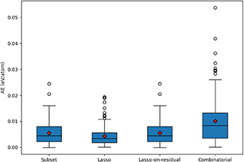
Figure 12. AE errors, in eV/atom, when applying different selectors in the CE model determination to CV. The horizontal line indicates 50% of the data (i.e. median) while the red diamond is the mean AE. All other colour and shape coding are the same as figure 10
Download figure:
Standard image High-resolution imageThe learning curves for the CE model training, as represented by the errors during the fit of the CE model and subsequent CV, are presented in figure 13 as a function of the sparsity (regularisation) parameter of the LASSO model (top) and as a function of the number of clusters used to fit the model (bottom). The optimal choices for the cluster size are when a minimum is attained in the test error curve (labelled cv-RMSE), as indicated with a red circle. As expected, low sparsity (i.e. a very large number of clusters) leads to small fit errors but an increase in CV errors, which is indicative of over fitting. Conversely, increased sparsity, which corresponds with very few clusters, lead to large errors in both the fit and the CV, indicating under fitting.
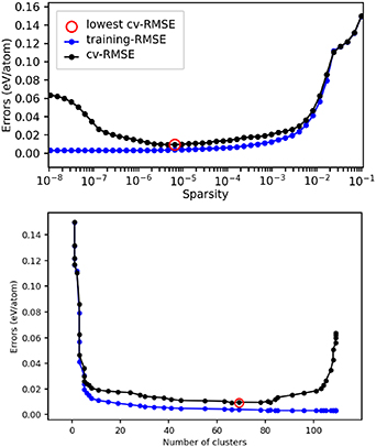
Figure 13. Plots of the error in training and CV for the FCC CE model as a function of sparsity (top) and number of clusters (bottom). The settings for the optimal model are highlighted with a red circle, and correspond to RMSE, MAE and MaxAE of 0.00349, 0.002 68, and 0.013 15 eV/atom, respectively, for the fit; and 0.005 64, 0.004 28, and 0.019 51 eV/atom, respectively, for the CV.
Download figure:
Standard image High-resolution imageTo conclude, the energy of mixing (Emix) is plotted in figure 14 as a function of Zn concentration for the ab initio DFT data on the FCC model, as well as the predictions from the training of the CE model, and the results when performing CV of the optimal model. The CE predictions are very good, showing accuracy of our model in most concentrations. The largest error is for 100% Zn, which is not a favourable FCC structure, and where the CV error is 0.019 eV/atom.
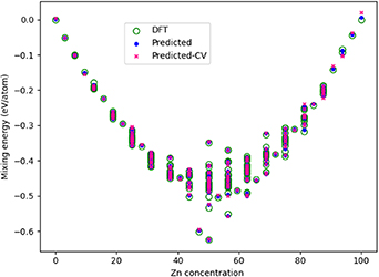
Figure 14. Plot of the mixing energy, Emix, as a function of Zn concentration, comparing the DFT results with those predicted from the CE model. A key is provided, with 'Predicted' referring to data included in the CE model training, and 'Predicted-CV' referring to predictions made on structures that were unseen during the CE model training.
Download figure:
Standard image High-resolution image4.2. HCP
For the HCP model, an equivalent parameterisation of the CE model was made with respect to dataset size, the size of the cluster pool, and the selector choice (see section 4.1.4). Filtering of the data was not necessary as structural distortion was not as prevalent as for the FCC system. The optimal model is obtained with the LASSO-on-residual selector, where the residual is computed considering a CE model that contains up to 3-body clusters, with a radius of 5 Å. The CE model error as a function of dataset sparsity and cluster pool size (Ncl ) are presented in figure 15.
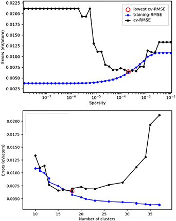
Figure 15. Plots of the error in training and CV for the HCP CE model as a function of sparsity (top) and number of clusters (bottom). The settings for the optimal model are highlighted with a red circle, and correspond to RMSE, MAE and MaxAE of 0.004 92, 0.004 00, and 0.014 41 eV/atom, respectively, for the fit; and 0.006 53, 0.005 14, and 0.021 10 eV/atom, respectively, for the CV.
Download figure:
Standard image High-resolution imageThe CE model predictions for mixing energy (Emix) are compared to ab initio DFT in figure 16. The predictions made for all Zn concentrations during the CV (red crosses) are generally close to the predictions when training the CE model (blue dots). The distribution of AE in the CV is presented as an insert box plot in figure 16. The predicted AE for the CV is below 0.012 eV/atom for most structures, as shown by the maximum value of the whiskers; only five outliers exist, with errors from 0.014 to 0.021 eV/atom. The MAE (red diamond) is 0.005 eV/atom.
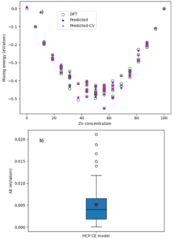
Figure 16. (a) Plot of the mixing energy, Emix, as a function of Zn concentration, comparing the DFT results with those predicted from the HCP CE model. A key is provided, with 'Predicted' referring to data included in the CE model training, and 'Predicted-CV' referring to predictions made on structures that were unseen during the CE model training. (b) A presentation of the distribution of the AE for the CV of the same HCP CE model. The middle horizontal line represents 50% of the data, with lower and higher whiskers representing the lower and upper bounds on the data.
Download figure:
Standard image High-resolution image5. Results and discussion
5.1. FCC
5.1.1. Coordination, Mulliken charges and density of states.
To understand the factors that control the energy of mixing (Emix) for PdZn alloys, the impact of Pd–Zn coordination was first considered for a range of predicted structures from the 1:1 stoichiometric alloy. As shown in figure 17, Emix increases with the number of unlike atoms in the first coordination shell, resulting in heterogeneous interactions, which agrees with the experimental observation for only ordered patterns to be synthesised [9, 10]. The heterogeneous coordination results in partial charge transfer, which are computed from DFT results and shown in the Mulliken charges in figure 18.
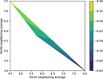
Figure 17. Heat map of Pd–Zn and Pd–Pd coordination effect. The colour bar shows the distribution of the mixing energy in eV/atom, with navy blue being the lowest (most favourable) mixing energy, and yellow the highest (least favourable) mixing energy.
Download figure:
Standard image High-resolution image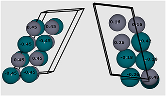
Figure 18. Mulliken charge (electrons, e) on Pd (blue) and Zn (purple) atoms for differing elemental distributions in PdZn stoichiometric alloys. The left structure has Emix of −0.625 eV/atom, and the right structure −0.349 eV/atom.
Download figure:
Standard image High-resolution imageFor the lowest energy structure with heterogeneous mixing of Pd and Zn in figure 18 (left), the Pd atoms are equally negatively charged with (–0.45 e) while Zn atoms are equally positively charged (+0.45 e). The more segregated ordering of Pd and Zn atoms in figure 18 (right) results in different charges of the two elemental species; Pd atoms are on average less negatively charged, ranging from −0.18 to −0.42 e, while Zn atoms are on average less positively charged, ranging from 0.16 to 0.48 e. For the less mixed system, charge transfer from Zn to Pd is greatest (−0.42 e) when the number of Zn atoms in the Pd coordination shell is large (8), and conversely charge transfer is smallest when the number of Pd–Pd interactions is largest. The increase in the charge transfer with the number of heterogeneous Pd–Zn interactions in the first coordination shell is a major factor behind the increase in Emix. The charge transfer will influence bulk and surface properties and could also affect the catalytic properties of the material [37]. The magnitude of the charge transfer between metal species is appreciable, with Mulliken charge transfer calculated with identical settings for Pd and Zn in their respective metal oxides, PdO and ZnO, i.e. Pd(II) and Zn(II), as +0.81 e and +1.17 e, respectively. For the 1:1 stoichiometric system, charge transfer is maximised for the ordered structure, which highlights the importance and stability of such elemental distribution, as well as potential importance for catalytic reactivity.
The calculated projected density of states (PDOS) for 3d electrons in the disordered and ordered stoichiometric PdZn, as well as Pd and Zn separately, are presented in figure 19. The 3d PDOS of pure Pd shows one large peak in the range of −5.5–0.5 eV, corresponding to near full occupancy of the Pd 3d shell. For Zn, the 3d orbitals contain a full 10 electrons, and thus the energy levels are from −7.0 to 0.0 eV, without a crossing of the Fermi level. For the mixed PdZn alloy with a disordered elemental distribution, the main 3d peak is shifted down to −7.5 eV, due to stabilisation of the Zn 3d electrons. Other peaks from −5.0 to −0.1 eV have Pd and Zn contributions (i.e. hybridised), though these states are also further from the Fermi level (figure 19(c)) than in pure Pd. For the ordered PdZn alloy (figure 19(d)), the position and intensity of the peaks are generally the same as for the disordered structure; however, the Pd 3d peak is positioned further from the Fermi level, stabilising this structure relative to the disordered alloy.
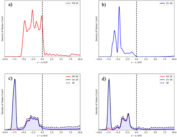
Figure 19. PDOS of (a) Pd, (b) Zn, (c) disordered PdZn, and (d) ordered PdZn. A legend is given on each image. The dashed vertical line is the Fermi level.
Download figure:
Standard image High-resolution image5.1.2. Phase diagram of FCC PdZn.
MMC simulations were performed with the CE model at 500 K for PdZn alloys, considering varying composition, with supercell sizes of  as well as
  and
and  . DFT optimisations were performed on the lowest energy structures observed in the MMC trajectory for the
  supercell, and for select
  supercells, with the DFT Emix results compared to that obtained from the CE model in figure 20.
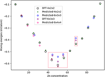
Figure 20. Comparison of the energy of mixing (Emix) as a function of Zn concentration when considering the most stable structures encountered in MMC simulations at 500 K (CE model) and subsequent DFT calculated energies (eV/atom). A key is provided. Note that the lowest Zn concentration plotted is 6.25%, and the highest is 93.75%.
Download figure:
Standard image High-resolution imageFor the  supercell, the Emix predicted from the CE model agree well with the DFT results, confirming the accuracy of the model. For the
  supercell, which contained 54 atoms, a local minimum search was undertaken with the CE model for 8 different concentrations, and 4 of these have been confirmed by DFT calculations (45%, 50%, 56% and 68.5% Zn, highlighted by pink rectangles on figure 20); concentrations of 13%, 26%, 82% and 87% Zn were also considered in the local minimum search with the CE model.
For the cross-comparison between CE model and DFT calculations for  supercells, the Emix predicted for 45% and 56% Zn agree well with DFT; however, an error of 0.04 eV/atom exists for 50% Zn (i.e. stoichiometric PdZn). The DFT optimised structure for the 1:1 PdZn model has angles and a lattice ratio deviating from the ideal FCC (x = 56.82° y = 56.512°, z = 68.52°, 2
  = 1.10 and 2
  = 1.01), which may explain the difference in Emix. A smaller error of 0.02 eV/atom is obtained for 68.5% Zn. Again, the error is attributed to distortion of the supercell from DFT optimisation; the orthorhombic phase is present in the experimental phase diagram at this Zn concentration, which corroborates with our observations. The angles distortions for 50% and 68.5% Zn concentration were outside the thresholds used when preparing the CE training dataset, and therefore were not suitable for re-training the CE model.
For both the  and
and  supercells, the lowest Emix is at 50% Zn. The GS configuration obtained for a
  supercell is reproduced with MMC simulations on the
  supercell; however, a new ordering is found for the
  supercell, as shown in figure 21. The
  GS structure has an average Pd-Zn coordination of 7.33, which is slightly smaller than the
  supercell (8); similarly, the average Pd-Pd coordination is slightly larger, at 4.67, when compared to the
  supercell (4). These changes in coordination result in an increase of Emix.
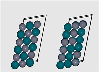
Figure 21. Left: GS configuration for a  supercell. Right: Disordered configuration at 1500 K, as considered during annealing. Pd and Zn atoms are represented by blue and grey spheres, respectively. Black lines indicate the cell boundaries.
Download figure:
Standard image High-resolution imageTo extend our simulations, we performed fully exhaustive enumeration of all possible structures, with all possible concentrations, with the CE model for supercells up to 12 atoms; extension to larger systems becomes rapidly intractable, and therefore the GS for large supercells can only be approached by performing MMC searches as explained prior. The method to fully enumerate over cell compositions is implemented in the CELL software package, based on the algorithm from Hart and Forcade [38]. The method generates all possible shapes of supercells with the specific numbers of atoms (1–12) resulting in 11 824 elemental configurations generated from the full enumeration. Emix for all these configurations are calculated with the CE model. The results of the full enumeration are shown in figure 22.
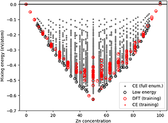
Figure 22. Energy of mixing compared with Zn concentration, considering full enumeration of all possible configurations with the FCC CE model. The grey dots represent the predicted energies for all possible structures up to 12 atoms. The red circles and red dots represent respectively the DFT data that forms the initial training dataset and the CE predictions on these same structures. The black circles represent the CE model predicted GSs at each concentration.
Download figure:
Standard image High-resolution imageCompared to the MMC search for larger supercells (figure 20), the GS had previously already been identified for Zn concentrations of 6.25%, 12.5%, 50%, 68.75%, 87.5% and 93.75%. For the other concentrations, longer MMC simulation runs would be necessary to reach the same GS.
5.1.3. Specific heat capacity.
The transition from the ordered GS of stoichiometric PdZn (the  -phase) to a disordered state has been considered for the
  supercell, as illustrated in figure 21. The mixing energy of the system has been collected from a MMC simulated annealing search using the CE model, with the temperature initial set to 3000 K and then decreased in steps of 500 K to 1 K, with 100 000 steps at each temperature. The specific heat capacity, Cp
, has been computed using equation (8), and is plotted against temperature in figure 23.
supercell, as illustrated in figure 21. The mixing energy of the system has been collected from a MMC simulated annealing search using the CE model, with the temperature initial set to 3000 K and then decreased in steps of 500 K to 1 K, with 100 000 steps at each temperature. The specific heat capacity, Cp
, has been computed using equation (8), and is plotted against temperature in figure 23.
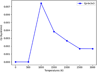
Figure 23. The specific heat capacity plotted as a function of temperature for a PdZn stoichiometric alloy, starting with GS ordering in a  supercell with 54 atoms.
Download figure:
Standard image High-resolution imageA peak in the specific heat capacity is observed at 1000 K, which indicates an order-disorder transition for the  supercell. A relatively high temperature is typical for stable or high entropy alloys [39]. Penner et al [40] reported changes to the ordered BCT PdZn structure (which is represented in our FCC CE model) at temperatures above 873 K. The high transition temperature aligns with experimental observations that the ordered structure is the only observed structure from synthesis when considering a 50% Zn concentration.
5.2. HCP
5.2.1. Phase diagram of HCP PdZn.
MMC simulations are performed using the HCP CE model for different  ,
,  and
and  supercells with a full range of Zn concentrations. Simulations were performed at 500 K with 500 000 steps, 600 000 steps and 800 000 steps, respectively, for the increasing supercell sizes. The results are displayed in figure 24.
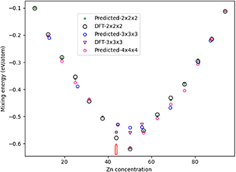
Figure 24. Comparison of the energy of mixing (Emix) as a function of Zn concentration when considering the most stable HCP structures encountered in MMC simulations at 500 K (CE model) and subsequent DFT calculated energies (eV/atom). A key is provided. The red arrow indicates a composition of 43.75% Zn, where DFT and CE models differ greatest.
Download figure:
Standard image High-resolution imageFigure 24 includes comparison between the most stable results from the MMC for the  supercell and DFT calculations subsequently performed on the same system. The results demonstrate that the HCP CE model correctly predicts the energies for most of the HCP structures. The largest difference between methods is 0.022 eV/atom for 43.75% Zn, as indicated by the red arrow in figure 24. The difference in Emix is attributed to distortion of the unit cell from DFT optimisation, with the structure tending towards the orthorhombic phase that is the most stable phase for these concentrations (figure 1).
For the  supercell, Emix is weaker than for the
  supercell when considering Zn concentrations of 45%, 50% and 56.5%; these results are confirmed by DFT calculations. For the
  supercell, the 50% Zn result matches the pattern observed for the
  supercell, indicating high stability. Overall, a pattern is observed whereby the GS configuration for even-numbered supercell expansions has Zn atoms adjacent to Pd atoms, maximising mixing; and for odd-numbered supercell expansions atom numbers, Emix is strongest when two atoms of the same species are adjacent to an alternative species atom, as shown in figure 25. Emix is strongest for PdZn (1:1), being −0.619 eV/atom, which is 0.005 eV/atom weaker than for the GS FCC structure with a 1:1 composition (−0.624 eV/atom). The difference in Emix increases if the chemical potential,
 , of the composite species is considered for the formation energy. The HCP phase has not been experimentally confirmed for the 1:1 concentration of PdZn, though it may be accessible using specific synthetic conditions such as low temperature. A study of how entropy contributes to the stability of the elemental orderings, and how relative phase stability changes with temperature, could provide further insight.
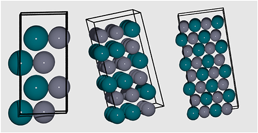
Figure 25. Schematic displaying the mixed pattern of atom positions obtained for low energy structures, considering the  (left),
  (centre) and
  (right) system, respectively.
Download figure:
Standard image High-resolution imageIn addition to the MMC simulations, a full enumeration for all HCP structures with up to 14 atoms was considered using the CE model. The resulting 60 107 configurations from the enumeration are presented in figure 26, which demonstrates that the MMC search (figure 24) coincides strongly with the full enumeration as the lowest energy structures are equivalent at several concentrations.
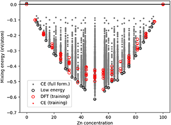
Figure 26. Energy of mixing compared with Zn concentration, considering full enumeration of all possible configurations with the HCP CE model. The grey dots represent the predicted energies for all possible structures up to 14 atoms. The red circles and red dots represent respectively the DFT data that forms the initial training dataset and the CE predictions on these same structures. The black circles represent the predicted GSs at every concentration.
Download figure:
Standard image High-resolution image5.2.2. Implications of the CE results.
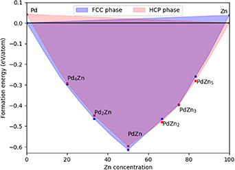
The formation energies (Efor) provide insight into phase diagram of PdZn and can be calculated by combining the chemical potential and the mixing energies, as shown in equations (5) and (6). The chemical potential  used for the FCC model is 0.036 eV/atom, while
  for the HCP model is 0.026 eV/atom. One can use the formation energy for each respective phase to construct a convex hull, which shows the predicted formation energies for FCC and HCP PdZn together (figure 27).
Figure 27. Overlay of convex hulls for formation energy (Efor) as a function of Zn concentration, representing the phase diagram of PdZn as produced by the CE models. The FCC and HCP regions are presented in blue and red, respectively. The most important FCC and HCP intermetallic alloys are denoted with blue and red dots, respectively.
Download figure:
Standard image High-resolution image
Considering first the pure Pd system, the FCC phase is favourable by 0.04 eV/atom compared to HCP. In the low Zn concentration range, the Pd2Zn phase was captured by the FCC CE model, highlighting the strong stability of the FCC phase below 50% Zn concentration. Depending on the experimental reduction conditions, Pd2Zn was observed as an intermediate during reduction of Pd/ZnO [41]; it exists in two different phases, namely, orthorhombic [13] and cubic [42].
At 50% Zn concentration, the FCC CE model, which includes the β-phase, predicts PdZn in the FCC phase to be more stable than HCP (by 0.017 eV/atom). The stable structure is the  -PdZn BCT model in its FCC representation, i.e. having c/a = 1.17/
 . Although the difference in Emix between the FCC and HCP representations is small, experimental synthetic conditions could explain the absence of HCP PdZn: α-PdZn (random FCC) and β-PdZn (ordered BCT) phases co-exist at all reduction temperatures considered in literature, suggesting that the α-PdZn phase is formed at lower Zn concentrations [9].
For higher Zn concentrations, the HCP phase is more stable generally. The experimentally observed orthorhombic PdZn2 structure is captured with the HCP CE model, which predicts PdZn2 to be more stable than the FCC phase (0.015 eV/atom). FCC PdZn3 is predicted to be more stable than HCP by a marginal 0.001 eV/atom, which is consistent with the XRD showing that this intermetallic alloy is in a cubic phase [43]. At larger Zn concentrations, HCP is predicted to be more stable in complete agreement with experiments [10], with the HCP phase favourable by 0.037 eV/atom for pure Zn. Future work may look at introducing CE models with an orthorhombic parent lattice, but this is beyond the scope of the current work.
6. Summary and conclusions
We have presented a detailed study that combines DFT and CE to understand the challenging experimental phase diagram of PdZn. We focused on three main crystallographic phases: FCC, HCP and BCT.
The models were trained with the energy of mixing, which was calculated using accurate DFT. CE models were built appropriately for the FCC and HCP phases; however, the BCT phase was unstable beyond stoichiometric PdZn, preventing creation of a model. For the FCC model, the training dataset was limited to structures that did not have deviation in the unit cell angles by >5° from the initial ideal FCC cell. For both the FCC and HCP CE models, the optimal CE model was obtained with the LASSO selectors. The GS structures were obtained by applying MMC searches in large supercells, and from full enumeration searches at smaller supercells.
By application of the CE model, a relationship was identified between Pd-Zn coordination and energy of mixing: the greater the heterogeneous coordination, the greater the mixing energy. Charge transfer, calculated with DFT, is greatest for these well mixed alloys, with electron transfer from Zn to Pd; this charge transfer may contribute to the catalytic reactivity of PdZn. Using the MMC approach, the GS configurations for the  FCC and a
  HCP supercells were identified as less stable than for
  and
and  FCC supercells, or
  and
and  HCP supercells, respectively.
For both FCC and HCP CE models, the 1:1 PdZn alloy has the lowest energy of mixing and represents the most stable structure on the convex hull. Insights into phase stabilities were obtained from the formation energies; for a 50% Zn concentration, the FCC phase (corresponding to the FCC representation of the  -phase) is 0.017 eV/atom more stable than the HCP structure. For all Zn concentrations <50%, the FCC structure is calculated to be more stable, while HCP is more stable for most Zn concentrations >50%. This observation is exemplified by Pd2Zn being more stable in the FCC phase, and PdZn2 being more stable in the HCP phase. A more accurate reproduction of the orthorhombic phases would require training a new CE model with structures generated with the orthorhombic parent lattice, which will be considered in future work.
Overall, our study shows that the CE approach can indeed describe the structure and key phases of the PdZn alloy. The ordered pattern for a concentration of 50% has been proven to be most stable compared to other ordering schemes. The outcomes will provide the basis for a new CE surface study of ordered PdZn.
Acknowledgments
The authors are grateful for funding by the EPSRC Centre-to Centre Project (Grant reference: EP/S030468/1), and the Project HPC-EUROPA3 (INFRAIA-2016-1-730897) supported by the E C Research Innovation Action under the H2020 Programme. S R, M T, and C A appreciate support from the Leibniz Science Campus GraFOx. We are grateful to Yuanyuan Zhou, Herzain Rivera, Luca Ghiringhelli, Matthias Scheffler, Martin Kuban, Graham Hutchings, and David Willock for useful discussions. A J L acknowledges funding by the UKRI Future Leaders Fellowship program (MR/T018372/1). The authors acknowledge computational resources and support from: the Supercomputing Wales project, which is part-funded by the European Regional Development Fund (ERDF) via the Welsh Government; the UK National Supercomputing Service YOUNG, accessed via membership of the Materials Chemistry Consortium which is funded by Engineering and Physical Sciences Research Council (EP/L000202, EP/R029431, EP/T022213); and the Isambard UK National Tier-2 HPC Service operated by GW4 and the UK Met Office, and funded by EPSRC (EP/P020224/1).
Data availability statement
The data that support the findings of this study are openly available from the NOMAD repository at DOI: 10.17172/NOMAD/2023.01.26-2 for the FCC structures and DOI: 10.17172/NOMAD/2023.01.26-1 for the HCP structures.
Conflict of interest
There are no conflicts of interest to declare.