Abstract
The magnetocrystalline anisotropy of GdRh2Si2 is examined in detail via the electron spin resonance (ESR) of its well-localised Gd3+ moments. Below TN = 107 K, long range magnetic order sets in with ferromagnetic layers in the (aa)-plane stacked antiferromagnetically along the c-axis of the tetragonal structure. Interestingly, the easy-plane anisotropy allows for the observation of antiferromagnetic resonance at X- and Q-band microwave frequencies. In addition to the easy-plane anisotropy we have also quantified the weaker fourfold anisotropy within the easy plane. The obtained resonance fields are modelled in terms of eigenoscillations of the two antiferromagnetically coupled sublattices. Conversely, this model provides plots of the eigenfrequencies as a function of field and the specific anisotropy constants. Such calculations have rarely been done. Therefore our analysis is prototypical for other systems with fourfold in-plane anisotropy. It is demonstrated that the experimental in-plane ESR data may be crucial for a precise knowledge of the out-of-plane anisotropy.
Export citation and abstract BibTeX RIS

Original content from this work may be used under the terms of the Creative Commons Attribution 4.0 licence. Any further distribution of this work must maintain attribution to the author(s) and the title of the work, journal citation and DOI.
1. Introduction
Besides exchange interactions and the distribution of magnetic moments the magnetocrystalline anisotropy is one of the most crucial aspects for understanding the magnetic properties of a magnetic material and notably its ground state. From a practical point of view, rare earth elements are used to increase the anisotropy of ferromagnets. In fundamental research the physics of 4f-electrons allows the study of a variety of phenomena, where strong spin–orbit interactions, helimagnetism, indirect exchange interactions and Kondo physics may be mentioned. In this work, the magnetocrystalline anisotropy of the tetragonal antiferromagnet GdRh2Si2 shall be in the spotlight, because previous works showed that its magnetism can excellently be described by a mean-field model together with an Ising-chain model [1] and it has been established experimentally that its anisotropy is well accessible by means of electron spin resonance (ESR) [2].
GdRh2Si2 belongs to the family of compounds with ThCr2Si2-structure which has provided an immense field for studying heavy-fermion physics including quantum phase transitions and Kondo effect [3, 4]. CeCu2Si2, CePd2Si2 and URu2Si2 show quantum criticality associated with the transition between antiferromagnetic and nonmagnetic ground states upon applying pressure. The suppression of antiferromagnetism is considered to induce unconventional superconductivity [5]. In YbRh2Si2, on the other hand, the antiferromagnetism with Néel-temperature TN = 65 mK [6] is suppressed by a small magnetic field and it has been suggested that its superconductivity below 2 mK is nonetheless the consequence of an antiferromagnetic instability at zero magnetic field [7]. While the g-factor is much larger in the tetragonal (aa)-plane than along the c-axis [8], suggesting an antiferromagnetic ground state order parameter within the plane, a precise experimental determination of this magnetic ground state is still lacking because of the weak magnetic moment and the low Néel-temperature [9, 10].
Considering this close structural and magnetic relation to YbRh2Si2, a thorough investigation of GdRh2Si2 by means of ESR seems even more interesting. The magnetic Gd3+-ions form stacked square lattice layers in the crystallographic (aa)-plane with the individual ions being in a tetragonal coordination. The exchange coupling within the layers is of ferromagnetic sign, but the coupling between the layers, thus along the c-direction, is antiferromagnetic. The magnetic structure is depicted in figure 1. As the magnetic moments only consist of the spin part (J = S = 7/2), no large spin–orbit interaction may be expected and the value of the saturated moment, μs = 7 μB, together with the lattice parameters yields a saturated sublattice magnetisation of Ms = 400 G. GdRh2Si2 has its Néel-temperature at TN = 107 K, allowing an easy experimental access to the ordered state.
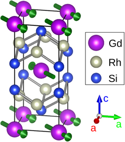
Figure 1. The tetragonal crystal structure of GdRh2Si2 with the magnetic structure of Gd ions illustrated [11] by the green arrows lying in the (aa)-plane.
Download figure:
Standard image High-resolution imageThe magnetic anisotropy aligns the spins into the (aa)-plane as has been explained by a detailed analysis of magnetisation measurements [1]. The major contribution to anisotropy is thus uniaxial and of easy-plane type. Additionally, a second, weaker anisotropy selects ground-state magnetisation directions within this plane, which are the [110]-, ![$\left[1\overline{1}0\right]$](https://content.cld.iop.org/journals/0953-8984/32/49/495801/revision2/cmabb17dieqn1.gif) -,
-, ![$\left[\overline{1}\overline{1}0\right]$](https://content.cld.iop.org/journals/0953-8984/32/49/495801/revision2/cmabb17dieqn2.gif) - and
- and ![$\left[\overline{1}10\right]$](https://content.cld.iop.org/journals/0953-8984/32/49/495801/revision2/cmabb17dieqn3.gif) -directions, see figure 1 for one possibility. On the other hand, this anisotropy term makes the spins to avoid the [100]-, [010]-,
-directions, see figure 1 for one possibility. On the other hand, this anisotropy term makes the spins to avoid the [100]-, [010]-, ![$\left[\overline{1}00\right]$](https://content.cld.iop.org/journals/0953-8984/32/49/495801/revision2/cmabb17dieqn4.gif) - and
- and ![$\left[0\overline{1}0\right]$](https://content.cld.iop.org/journals/0953-8984/32/49/495801/revision2/cmabb17dieqn5.gif) -directions. This minor anisotropy contribution is consequently of fourfold symmetry around the c-axis. As it is responsible for the spin direction within the (aa)-plane, it is termed basal anisotropy. Due to the four possibilities for the magnetisation sublattices to align within the basal plane in zero and low magnetic fields, a domain structure is developed [1]. Thus, figure 1 shows only one of the magnetic domains and the other three domains are obtained by rotating all the depicted spin vectors by 90°, 180° or 270° about the c-axis. The ESR in GdRh2Si2 could be followed far inside the ordered regime [2], both at X-band and Q-band frequency. High-field ESR therefore seems unnecessary in this system and it is the aim of this work to quantify both terms of magnetocrystalline anisotropy at several temperatures T < TN using a conventional ESR setup. In our ESR experiments, especially in all the Q-band experiments, the magnetic fields of interest are large enough to have only one single antiferromagnetic domain. Hence, the domain suppression effects do not disturb the evaluated resonances.
-directions. This minor anisotropy contribution is consequently of fourfold symmetry around the c-axis. As it is responsible for the spin direction within the (aa)-plane, it is termed basal anisotropy. Due to the four possibilities for the magnetisation sublattices to align within the basal plane in zero and low magnetic fields, a domain structure is developed [1]. Thus, figure 1 shows only one of the magnetic domains and the other three domains are obtained by rotating all the depicted spin vectors by 90°, 180° or 270° about the c-axis. The ESR in GdRh2Si2 could be followed far inside the ordered regime [2], both at X-band and Q-band frequency. High-field ESR therefore seems unnecessary in this system and it is the aim of this work to quantify both terms of magnetocrystalline anisotropy at several temperatures T < TN using a conventional ESR setup. In our ESR experiments, especially in all the Q-band experiments, the magnetic fields of interest are large enough to have only one single antiferromagnetic domain. Hence, the domain suppression effects do not disturb the evaluated resonances.
The theoretical description of the anisotropy shall be by the classical theory of antiferromagnetic resonance where the eigenfrequencies of two coupled, oscillating magnetisation sublattices are evaluated. More precisely, we are mainly interested in resonance fields of our ESR data for a given oscillation frequency. Nevertheless, calculated resonance frequencies as a function of external field are presented at the end of this report, giving additional insight into antiferromagnetic resonance in the presence of both uniaxial and fourfold basal anisotropy.
2. Methods
2.1. Sample preparation
The growth of the single crystals of GdRh2Si2 and their characterisation are explained in reference [12]. We used a platelet shaped sample with an area of about 1 × 1.3 mm2 and a thickness of about 0.5 mm.
2.2. ESR spectroscopy
Continuous-wave ESR was performed both at a frequency of νrf = 34 GHz (Q-band) and at 9.4 GHz (X-band). A Bruker Elexsys II spectrometer was used. In case of the Q-band experiments the resonator was a cylindrical Bruker ER5106QTW cavity and for X-band measurements the resonator used was a rectangular Bruker ER4122SHQ. In both cases a helium gas-flow cryostat allowed a temperature stability of less than 1 K. To measure the angular dependence in the naturally grown (aa)-plane, the samples were mounted with their growth plane perpendicular to the rotation axis of a goniometer. In order to perform rotations in the (ac)-plane, an a-axis was aligned parallel with the rotation axis, the sample being glued on a vertical facet of a glass holder. The external field H0 was swept up to 1.8 T. The spectra shown in this work are the first derivative of the absorbed microwave power, owing to the use of lock-in technique with field modulation.
2.3. Anisotropy simulations
Looking for the eigenoscillations of two antiferromagnetically coupled magnetisation sublattices, these two magnetisations are written as  with i = 1, 2, meaning a decomposition into their static parts (index 0) and dynamic parts (small letters), where
  . Their equations of motion read


Here,  and
and  are the static and dynamic effective fields acting on the respective sublattice i with
  , and γ is the gyromagnetic ratio. Equations (1) and (2) are derived from the respective Landau–Lifshitz equations by linearising in the small quantities m(i) and
  and by setting the damping to zero [13]. Effective fields are expressed via the free energy density F:
where α and β denote Cartesian components x, y, z. The internal energy in the system to be investigated by ESR consists of exchange energy Fe, Zeeman energy FZ, uniaxial anisotropy energy Fu and basal anisotropy energy Fb:
Here, Λ is the dimensionless antiferromagnetic exchange constant, H0 the external magnetic field, Ku the first order uniaxial anisotropy constant and Kb the first order basal anisotropy constant. The definitions of the polar angles θi correspond, in figure 2(a), to the angles between the M(i) and the axis of uniaxial anisotropy (z-axis), and the azimuthal angles φi are, as is illustrated in that same sketch, defined within the (aa)-plane. Note that the above definition of basal anisotropy energy matches the one in reference [1].
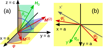
Figure 2. (a) Illustration of the field and magnetisation geometry when the external field H0 is within the (ac)-plane [here: (yz)-plane]. The external field spans an angle of θH with the z-axis. Sublattice magnetisations M(1) and M(2) lie symmetrically with respect to the (yz)-plane. Their common plane (violet) defines the angle θ' to the z-axis, which is not the same as the angle θ := θ1 = θ2 spanned between the M(i) and z. The basal anisotropy energy is defined via the azimuthal angle φ within the (aa)-plane, and in the case shown φ := φ1 = φ2. (b) For the field within (aa)-plane, it is convenient to define y' ∥ H0. φ1' and φ2' are then measured against the x'-axis. φH is measured between H0 and the y-axis.
Download figure:
Standard image High-resolution imageWith  and z0 as the unit vector along z, the effective fields are, again after linearising in the m(i),
The effective fields of basal anisotropy,  and
and  , will be explained below for the two cases of field rotation separately. Equations (1) and (2) define in this way a coupled linear equation system, with six independent variables, namely the three Cartesian components of the two dynamic magnetisations m(i). Defining a 6 × 6-matrix A, this is summarised as

In order to get nontrivial solutions, we set det A = 0, providing either resonance frequencies νres for a given field or resonance fields Hres for a given microwave frequency. Of particular interest are two special cases, for which (6) is solved analytically [13] for Ku < 0 as is the case in GdRh2Si2: firstly, when Kb = 0 and H0 is in the basal plane, one of the two resonance frequencies is

where H0 = |H0|. This value is very close to the paramagnetic value ωres = γH0 as long as the exchange field ΛM0 is large as compared to the anisotropy field Hu = 2Ku/M0. Secondly, for Kb = 0 and with H0 along the c-axis, one of the resonances occurs at ωres = 0, corresponding to a Goldstone mode, which is provided from the spontaneous symmetry breaking by the antiferromagnetic order parameter.
2.3.1. Out-of-plane rotations
When rotating the field within the (ac)-plane, and as long as we deal with the static field and magnetisation parts only, we may benefit from the mirror symmetry with respect to the (ac)-plane (see figure 2(a)) and write θ = θ1 = θ2 as well as φ = φ1 = φ2. For further calculations, it is convenient to introduce a primed coordinate system x', y', z' with x' = x, but tilted by the angle 90° − θ' towards H0, having y' within the purple plane of figure 2(a) and z' perpendicular to it. Now we introduce the angles  , θ' = ∢(y', z) and
  . The relationships between convenient angles θ', φ' and the angles θ, φ and δ used in (4) read
In this way, the free energy is expressed in terms of θ' and φ' as
The two equilibrium angles θ0' and φ0' are found via the minimum of F.
When setting up the matrix A as defined by (6), however, the two sublattices with the respective effective fields acting on them need to be treated separately and the contracted form (9) for F is not suitable. Moreover, F shall be represented in a Cartesian form. In the primed coordinate system,  ,
,  ,
,  , z0 = (0, cos θ0', sin θ0') and the calculation of the matrix A using the equations of motion (1), (2) and the effective fields (5) is straightforward, except for the basal anisotropy fields.
With  in the unprimed system and
  in the primed system we have
  ,
,  . From figure 2(a) follows
Note that now φi stands for the azimuthal angle due to both static and dynamic magnetisation parts. The two parts i of the basal anisotropy energy Ub in (4) are then expressed in a Cartesian way as
where static and dynamic magnetisation parts are still unseparated. Effective field components  in direction α' are obtained as
  . Magnetisation components are subsequently separated into static and dynamic parts. Following (3), the static parts of the field components
  are given by setting m = 0 and the dynamic field components
  are obtained as linearisations in the
  . The assumption
  , reflecting that the exchange field is the dominating interaction gives important simplifications. Concerning the static parts of the two sublattices, the only difference between them is the reversed static x-component:
  .
.
The resulting terms needed for the calculation of θ0', φ0' and A are documented in appendix
2.3.2. In-plane rotations
Following figure 2(b), the primed coordinate system is now defined by z' = z, but with y' ∥ H0, being thus rotated by the angle φH around z with respect to the unprimed framework. The static part of the total magnetic energy may be written
Now the equilibrium angles  and
and  are found as the ones minimising F.
In the primed coordinate system H0 = (0, H0, 0),  and
and  . As before, exchange, Zeeman and uniaxial terms in (1), (2) and (5) can be easily calculated. The basal anisotropy energy shall again be expressed in terms of Cartesian magnetisation components, so that basal terms can be introduced into matrix A, too. The angles φ1' and φ2' are regarded as due to both static and dynamic magnetisation. The Kb-term in (12) is expanded into sines and cosines of only φ1' or φ2', and using the just mentioned representations of the
  , the basal energy parts become
Here again, Hbα' = −∂U/∂Mα'. The procedure is then completely analogous to the out-of-plane treatment: separation into static and dynamic magnetisations, determination of effective fields as described by (3) using approximations  and construction of A's matrix entries following (1), (2), (5) and (6). Note that, unlike the out-of-plane case, in general
  and
and  .
.
Appendix  ,
,  and A.
2.3.3. Numerical procedure
When plotting resonance frequencies against magnetic field, it is sufficient to once calculate the equilibrium directions of sublattice magnetisations for given parameters and subsequently compute the resonance frequency. It turned out to be helpful to start with the highest field and then reduce the field in the plot, because at lowest fields other solutions than the physically observed ones may be captured as will be discussed below. When plotting resonance fields versus a field angle (either θH or φH) for a given microwave frequency, equilibrium directions and resonance fields need to be computed iteratively, because magnetisation directions depend on the resonance field and vice versa.
In either case the starting point for the resonance condition is the analytical expression (7), which is valid for H0 ∥ a and Kb = 0. Therefore, calculations start with these parameters and the first field angle (other than θH = 90°, φH = 0°) as well as Kb are switched on in small steps. Azimuthal angles φ' are initialized with the value H0/(ΛM0).
Zeros of det A, providing the resonance condition, as well as the zeros of (9) and (12), providing equilibrium angles, are implemented by the (one-/two-dimensional) Newton method. The derivatives of det A are computed by difference approximations either in ω or H0. The derivatives needed for equilibrium angles are given analytically in the appendix.
3. Results and discussion
3.1. ESR anisotropy in the ordered regime
A few representative ESR spectra from the antiferromagnetically ordered state in GdRh2Si2 are plotted in figure 3, showing the field derivative of the absorbed microwave power, dPabs/dH0, versus the external field H0. The fits use an asymmetric Lorentzian derivative, where the asymmetry is due to the conductivity of the sample [2]. The asymmetric lineshape indeed physically makes sense, because the penetration depth amounts to about 3 μm in the paramagnetic regime [14], much smaller than the thickness of the sample of about 0.5 mm. A dropping resistivity below TN towards about 3 μΩcm at T = 5 K [12] results in even smaller penetration depths in the ordered state. It is seen that these fits provide an excellent description of the measured spectra, confirming the idea of well-localised and strong Gd3+ magnetic moments. Obtained parameters are the resonance field Hres, the linewidth ΔH, the asymmetry ratio D/A and the line intensity I, which corresponds to the area under the non-derived spectrum. While the focus shall here be on the resonance fields, it is noteworthy that the linewidth, in the range of 400 Oe, typically increases with increasing resonance field, as is also observed in the ordered states of many other localised-moment magnets [15–17]. D/A mostly assumes values between 0.5 and 1.0, in accordance with the expectation for a conductive system. Concerning Hres, a clear anisotropy is distinguished when rotating the external field out of plane (left frames in figure 3), but also within the (aa)-plane (right frames). The figure demonstrates that decreasing temperature enhances the magnetocrystalline anisotropy, which is because the sublattice magnetisations approach their saturated values.
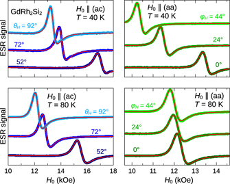
Figure 3. Q-band ESR-spectra of the GdRh2Si2 single crystal. The static magnetic field was rotated in the (ac)-plane (left frames) and in the (aa)-plane (right frames). The temperature of 40 K (upper frames) is compared to the temperature of 80 K (lower frames). Solid lines: fit curves by a single asymmetric Lorentzian derivative.
Download figure:
Standard image High-resolution imageThe resonance fields for out-of-plane rotations at different temperatures are shown in figure 4. At the temperature of 80 K and at θH = 90°, meaning that the field is along the a-axis, the resonance field amounts to 12.2 kOe, close to the value of 12.1 kOe given for a paramagnetic moment with g = 2 at the frequency νrf = 34 GHz. Following (7), which holds for this field direction as long as basal anisotropy is negligible and when uniaxial anisotropy is much smaller than the exchange field, the paramagnetic value is indeed expected here. Resonance fields diverge when approaching H0 ∥ c and the observation of the resonance gets limited by the largest possible external field. As the resonance fields increase with decreasing temperature, only an angular range of ±30° around the a-axis is covered at T = 20 K. Diverging resonance fields for H0 ∥ c indicate that for a fixed external field the resonance frequency gets suppressed down to zero, thus reaching the Goldstone mode which cannot be observed experimentally. We can conclude that the quasi-paramagnetic mode at θH = 90° in easy-plane antiferromagnets with resonance condition (7) transforms continuously into the Goldstone mode also mentioned in section 2.3 when tilting towards the hard axis. Resonance fields at T = 5 K were analyzed, too, but are not displayed here because of a vanishing ESR signal over a wide angular range.
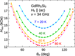
Figure 4. Q-band resonance fields from rotations within the (ac)-plane at temperatures between 20 and 80 K. θH = 0° means H0 ∥ c and θH = 90° corresponds to H0 ∥ a. Solid lines: fits to the measured data, see main text and the fit parameters in figure 6(a).
Download figure:
Standard image High-resolution imageFit curves in figure 4 demonstrate that the theoretical model of coupled oscillating magnetisation sublattices satisfactorily describes the measured data. Free fit parameters are only Ku and Kb and the g-factor is fixed to g = 2. Other parameters, which are supplied by external measurements, are the microwave frequency νrf, the sublattice magnetisations M0 and the exchange constant Λ. We calculate the temperature dependence of M0 as  with the saturation value Ms = 400 G which one gets for the Gd3+ moment μ = 7 μB using lattice constants given in reference [12]. Λ can be calculated within a mean-field theory from the Néel-temperature TN, the Curie–Weiss-temperature ΘCW and the Curie constant C as Λ = (TN + ΘCW)/C = 710 [18]. The fitted anisotropy constants are discussed in section 3.2.
In-plane resonance fields are shown in figure 5. Here, a fourfold anisotropy is clearly visible. From the point of view of the uniaxial anisotropy, the (aa)-plane is an easy plane, but the additional basal anisotropy changes the a-axes (φH = 0°, 90°) into hard axes within this plane, whereas the [110]-axes are the easy axes. Thus, according to the definition in (4), Kb is negative in GdRh2Si2. As in the out-of-plane case, the anisotropy simulations fit the experimental data very well over a broad temperature range between 20 and 80 K. This is the case for T = 5 K, too, but the data are not shown here due to spectra of bad quality over a wider angular range. As before, the free fitting parameters are Ku and Kb only.

Figure 5. Q-band resonance fields from rotations within the (aa)-plane at temperatures between 20 and 80 K. φH = 0° means H0 ∥ a. Solid lines: fits to the measured data, see main text and the fit parameters in figure 6(b). High temperature and low temperature data are shown separately due to the different ordinate scales.
Download figure:
Standard image High-resolution imageESR data were additionally recorded at X-band microwave frequency. The resonance fields generally reflect the same behaviour as described above for the Q-band. The spectra can be well evaluated for temperatures T > 60 K. At lower temperatures, the signal weakens and gets disturbed by nonresonant low-field features in the spectra [2] due to a spin–flip transition aligning the magnetic sublattices from their ground state configuration to nearly perpendicular to the external field [1]. For 60 K and 80 K, we applied the parameters from the Q-band fits to the frequency of 9.4 GHz. Whereas the agreement to experimental data at 80 K is still acceptable, the simulation does not match the X-band data at 60 K. While the experimental data has, for rotations in the (aa)-plane, its minima at 1800 Oe, the simulation drops down to less than 600 Oe, where it becomes discontinuous. Section 3.3 takes up this issue in more detail.
3.2. Anisotropy constants of GdRh2Si2
Figure 6 summarises the anisotropy constants determined from the fits in section 3.1. Both kinds of field rotations provide an uniaxial constant Ku in the same order of magnitude, see figure 6(a). Rotations in the (aa)-plane seem more trustworthy, because they reproduce, except for the lowest temperature, a monotonous increase with decreasing temperature. Surprisingly, out-of-plane rotations, i.e. in the (ac)-plane, only suggest a rather constant Ku over the given temperature range and are, thus, considered less suitable for providing the uniaxial anisotropy constant. Indeed, the divergence of Hres towards the c-axis (see figure 4) is an intrinsic feature of easy-plane antiferromagnets and in first respect is not dependent on the magnitude of the negative Ku. Error bars in figure 6 are roughly estimated by variation of the respective anisotropy constant until the square deviations χ2 of the fit get doubled. Thus, they indicate the borders where deviations in K would result in a similar error in the fit as compared to the remaining χ2 at its minimum. Obviously, for Ku there is no satisfactory overlap between (aa)- and (ac)-measurements at 60 and 80 K. On the low-temperature side, the result for 5 K must even more be considered with caution. Experimentally it was difficult to obtain an ESR signal of reasonable strength at this temperature and it even was weakened further during both kinds of rotations, so that we could only access limited angular ranges. The reason therefore could not be clarified. Thus, we consider at least the value obtained for Ku at the lowest temperature unlikely and the seeming maximum at 20 K shall not be taken too serious. The neglection of the point at 5 K would allow an extrapolation of the more reliable (aa)-data to an order-of-magnitude estimation of the lowest-temperature value Ku ≈ −10 × 106 erg cm−3, corresponding to an anisotropy field Hu = |2Ku/M| = 50 kOe. As shown by figure 6(a), a precise determination of Ku in this system is generally hard to be realized by antiferromagnetic resonance. The reason why especially the (ac)-fits do not allow a satisfactory determination of Ku is that, contrary to the expectation, large variations of this constant only lead to a minor vertical shift of calculated resonance fields in figure 4. The main contribution to the shifts stems from the basal anisotropy constant Kb. The divergence of Hres towards H ∥ c is characteristic for the considered type of antiferromagnet, irrespective of the detailed size of Ku, as long as Ku < 0. The fact of minor vertical shifts of calculated Hres upon large modification of Ku has been proven in the in-plane plots Hres(φH) (figure 5), too. This is the reason, why also the (aa)-points in figure 6(a) partially have large errors.
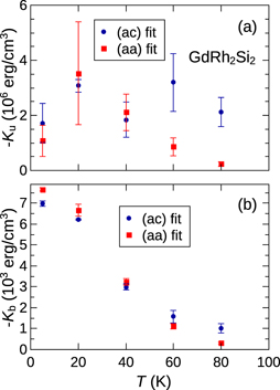
Figure 6. (a) The negative of the uniaxial anisotropy constant Ku in GdRh2Si2. (b) The negative of the basal anisotropy constant Kb. In both cases the results from in-plane and out-of-plane measurements are compared. See the main text for the definition of error bars.
Download figure:
Standard image High-resolution imageConcerning the physical origin of anisotropy in GdRh2Si2, several mechanisms may be mentioned. Because of the spin-only magnetic moments of Gd3+ (ground state 8S7/2), admixtures of excited atomic states are needed to account for a possible single-ion anisotropy, which however would only explain an anisotropy field less than 0.1 kOe and a similar estimate is obtained for the anisotropy due to dipolar interaction [19]. Instead exchange anisotropy as a microscopic origin of anisotropy has been discussed in the literature [19, 20].
Contrary to Ku, it must be noted that the basal anisotropy constant Kb (figure 6(b)) is generally more consistent between both kinds of measurements, out-of-plane and in-plane rotations. Error bars are small in the latter case. At 80 K the drop of Kb as determined by the (aa)-plane experiments seems more realistic and makes these measurements again preferable over the (ac)-plane experiments. And indeed it is considered natural that in-plane-rotations provide the basal anisotropy constant much more accurately. Nevertheless it is surprising that also the out-of-plane measurements give rather accurate results for the strength of the basal anisotropy. At low temperatures, Kb amounts to approximately −7000 erg cm−3. The smallness of the basal anisotropy as compared to the dominant uniaxial term is worth to note and the reason why it is usually neglected [13].
3.3. Calculated resonance frequencies
Pure simulations of resonance frequencies νres as a function of external field H0 are plotted in figure 7. M0 = 400 G and Λ = 710 are chosen as the low-temperature parameters for GdRh2Si2, Ku = −1 × 10⁶ erg cm−3 is taken in an order of magnitude realistic for GdRh2Si2 as well as g = 2. In figure 7(a) the field angles θH = 70° and φH = 0° are selected and Kb, the anisotropy parameter which is mainly discussed in this work, is varied in steps of 1000 erg cm−3. Starting with Kb = 0 a proportionality between H0 and νres is observed with a slightly smaller slope than one would expect for a g = 2 paramagnet. That slope, however, is almost restored when setting θH = 90° (not shown in the figure), as can be seen from (7). When turning Kb positive, zero field resonances occur at finite frequencies, meaning that an excitation gap opens. This is because for positive Kb the easy axes of the basal anisotropy are along the a-axes, which also correspond to the approximate magnetisation directions in our calculation. Thus even at zero external field the sublattice magnetisations underlie the existing internal anisotropy field, yielding finite resonance frequencies at H0 = 0. For Kb < 0 the curves in figure 7(a) bend in the opposite way and for low external fields the simulations fail. A spin reorientation transition takes place. At zero and low external fields the sublattice magnetisations are, in reality, along the diagonals between the a-axes. With increasing H0, the M(i) turn continuously towards directions close to the a-axes and νres decreases, because internal and external fields counteract. When the magnetisation has become perpendicular to the external field, the resonance frequency can again increase with increasing field which is indeed seen in the simulations. As our model is based on the latter magnetisation configuration, the low field features are not captured in figure 7(a). Empirically, the excitation gaps for Kb > 0 observed in this figure match the well-known expression  [13], when defining the basal anisotropy field as
  .
.

Figure 7. Plots of calculated resonance frequencies νres versus external field H0 for variation of different parameters. (a) The field direction is at the polar angle θH = 70° within the (ac)-plane and the basal anisotropy Kb is varied in steps of 1000 erg cm−3. (b) θH is rotated within the (ac)-plane. (c) The azimuthal field angle φH is rotated within the (aa)-plane. In all three cases the uniaxial anisotropy Ku = −1 × 10⁶ erg cm−3. In frames (b) and (c), Kb = −5000 erg cm−3.
Download figure:
Standard image High-resolution image
The situation is similar in figure 7(b), where Kb = −5000 erg cm−3 is fixed and the angle θH of the external field within the (ac)-plane is varied. The spin-reorientation transition is always observed, but its field value increases when tilting H0 away from the (aa)-plane. Moreover, the resonance frequency above this transition gets more and more suppressed. At θH = 0° one ends up with the aforementioned Goldstone mode νres = 0. In figure 7(c) the same anisotropy constants are used, but the rotation now takes place within the (aa)-plane. For φH = 0° the same situation as in figure 7(b) at θH = 90° is encountered. Increasing to φH = 1° already lifts the minimal resonance frequency from 0 to 10 GHz, rendering the simulations possible even below the transition. The significant difference to out-of-plane simulations is here, that the azimuthal angles of the two sublattice magnetisations may differ from each other when employing in-plane simulations. As anticipated before, νres-curves in figure 7(c) approach a constant and finite value at zero field. The upwards trend is continued up to φH = 45°, where the situation now corresponds exactly to the case of φH = 0° and Kb = +5000 erg cm−3 in figure 7(a).
These field-frequency plots help to understand why the X-band data on GdRh2Si2 are not suitably described by our model. With too large anisotropy constants, the excitation gap is not overcome by the microwave energy. At higher temperatures, anisotropies are small and the excitation gap may still be overcome. But even then, the steep slopes in νres(H0) when the external field is in the (ac)-plane or close to it as well as strong shifts of Hres at νrf = 9.4 GHz during field rotations destabilize the simulation.
4. Conclusions
From an application point of view, magnetic anisotropy gets its largest interest in magnetic thin films and bulk ferromagnets. Here, ESR is an important tool for its determination. The anisotropy in bulk antiferromagnets, however, is mostly measured by macroscopic magnetisation measurements, because typically the experimental access by ESR is difficult. With this work we could demonstrate that there are cases where the anisotropy in an antiferromagnet can nevertheless be well measured by conventional ESR. In GdRh2Si2, the angular dependences of resonance fields at Q-band frequency are excellently fitted by the model of two oscillating magnetic sublattices, using only two free parameters. The specific type of magnetic anisotropy includes an easy-plane uniaxial and an additional fourfold basal term. The uniaxial term is dominant with an anisotropy field at low temperatures of the order Hu ≈ 50 kOe. With small uncertainty, we could quantify the basal anisotropy constant at low temperatures to Kb ≈ −7000 erg cm−3, giving by definition a basal anisotropy field of  . Supported by the agreement between experimental data and calculated resonance fields, it was safe to plot theoretical field-frequency diagrams which essentially support the idea of the basal anisotropy leading to an excitation gap and, depending on its sign or the field direction, possibly to a spin–flip transition. It turned out that magnetocrystalline anisotropy alone is sufficient to describe ESR angular dependences, whereas we did not find clear indications for a possible anisotropy of the g-factor.
This experimental study and the excellent agreement between our theoretical modelling and the experimental results demonstrate that in magnetic systems with easy plane behaviour and weak in-plane anisotropy ESR experiments can provide a deep insight into anisotropic properties and interactions. On a more general level, we would like to emphasize that it is reasonable and worthwhile not only to consider the dominant uniaxial anisotropy, but also the weaker in-plane anisotropy. Our results provide a basis for the study and analysis of such systems. One of the most interesting candidates is the system YbRh22Si2. This sister compound to GdRh2Si2 is located extremely close to a quantum critical transition between an antiferromagnetic and a paramagnetic ground state. This results in very unusual properties, e.g. strong deviation from Fermi liquid behaviour, as well as a unique electronic–nuclear transition to a superconducting state. Therefore YbRh2Si2 has attracted very strong interest. However, because the size of the ordered moment is extremely small, of the order of 10−3 μB, and the ordering temperature is pretty small too, TN = 70 mK, most of the characteristics of the AFM state are yet not clear. Fortunately YbRh2Si2 is an easy plane system with weak in-plane anisotropy as GdRh2Si2, and surprisingly a well-defined ESR can be observed despite the presence of a strong Kondo interaction [21]. Moreover, in preliminary experiments using a broad band technique, this ESR signal could be followed down to very low temperatures and low magnetic fields, well into the AFM state. Extending these experiments and analyzing the spectra using the models and knowledge developed in the present study on GdRh2Si2 shall likely allow to get much deeper insight into the magnetism and AFM state of YbRh2Si2, and thus provide important information to get an understanding of this paradigmatic quantum critical system.
Acknowledgments
DE appreciates the inspiring discussions with H-A Krug von Nidda.
Appendix A.: Formulae for out-of-plane rotations
The formulae are in the primed framework of figure 2(a). Differing from the main text however, the primes of θ' and φ' are omitted here for better readability. The angles θ and φ in this appendix shall not be confused with θ and φ from the main text.
A.1. Equilibrium angles
where D = 1 − cos2 θ sin2 φ.
A.2. Elements of matrix A
Using  ,
,  , η:=My0 sin θ/Mx0, ωe := γΛM0, ωu := 2Kuγ/M0 and
  , the matrix elements are
and further A43 = A16, A45 = A12, A46 = A13, A53 = A35, A54 = A21, A56 = −A23, A61 = A34, A62 = A26, A64 = A31, A65 = −A32 as well as A14 = A15 = A24 = A25 = A36 = A41 = A42 = A51 = A52 = A63 = 0. The coefficients kαβ, connecting dynamic magnetisation component β to dynamic basal field component α are
and kyx = kxy, kzx = kxz, kzy = kyz.
Appendix B.: Formulae for in-plane rotations
The formulae are in the primed framework of figure 2(b). Differing from the main text however, the primes of φ1' and φ2' are omitted here for better readability. The angles φ1 and φ2 in this appendix shall not be confused with φ1 and φ2 from the main text.
B.1. Equilibrium angles
B.2. Elements of matrix A
Using  ,
,  ,
,  ,
,  , ωe := γΛM0, ωu := 2Kuγ/M0 and
  , the matrix elements are
and further A11 = A22 = A33 = A44 = A55 = A66 = iω, A12 = A14 = A15 = A21 = A24 = A25 = A36 = A41 = A42 = A45 = A51 = A52 = A54 = A63 = 0 as well as A34 = −A16, A35 = −A26, A61 = −A43, A62 = −A53. Static basal field components and dynamic basal coefficients for the two sublattices i = 1, 2 are