
Abstract
Colorectal cancer (CRC) is the 3rd most common and the 2nd most deadly type of cancer worldwide. Understanding the biochemical and microstructural aspects of carcinogenesis is a critical step towards developing new technologies for accurate CRC detection. To date, optical detection through analyzing tissue chromophore concentrations and scattering parameters has been mostly limited to chromophores in the visible region and analytical light diffusion models. In this study, tissue parameters were extracted by fitting diffuse reflectance spectra (DRS) within the range 350–1900 nm based on reflectance values from a look-up table built using Monte Carlo simulations of light propagation in tissues. This analysis was combined with machine learning models to estimate parameter thresholds leading to best differentiation between mucosa and tumor tissues based on almost 3000 DRS recorded from fresh ex vivo tissue samples from 47 subjects. DRS spectra were measured with a probe for superficial tissue and another for slightly deeper tissue layers. By using the classification and regression tree algorithm, the most important parameters for CRC detection were the total lipid content (flipid), the reduced scattering amplitude (α'), and the Mie scattering power (bMie). Successful classification with an area under the receiver operating characteristic curve higher than 90% was achieved. To the best of our knowledge, this is the first study to evaluate the potential tissue biomolecule concentrations and scattering properties in superficial and deeper tissue layers for CRC detection in the luminal wall. This may have important clinical applications for the rapid diagnosis of colorectal neoplasia.
Export citation and abstract BibTeX RIS

Original content from this work may be used under the terms of the Creative Commons Attribution 4.0 license. Any further distribution of this work must maintain attribution to the author(s) and the title of the work, journal citation and DOI.
1. Introduction
Colorectal cancer (CRC) is the 3rd most common type of cancer worldwide (11.3% of the diagnosed cancer cases in 2020) and 2nd most deadly (10.2% of the cancer related deaths in 2020) [1, 2]. There is an increasing emphasis on early detection of CRC and this is usually associated with a good outcome. With this in mind, screening and diagnostic tests (e.g. stool tests, flexible sigmoidoscopy and colonoscopy) have a positive impact in decreasing CRC death rates, especially by incorporating newer and more sophisticated endoscopic imaging modalities [3, 4]. Colonoscopy involves inserting an endoscope into the large bowel to visualize the colonic and rectal mucosa directly. The goal of colonoscopy is not only to detect cancer, but also to detect and remove benign neoplastic polyps with malignant potential, thus reducing the subsequent incidence of cancer. However, the sensitivity and specificity for the detection of premalignant polyps during conventional white-light colonoscopy are 82.9% and 80.0%, respectively [5], whereas, even small cancers can be overlooked particularly with flat lesions in the caecum and ascending colon [6–11].
Currently, the gold standard for the characterization of polyps is histopathology, but this is not available in real time. False classification of innocuous polyps as benign or malignant neoplasia at colonoscopy will lead to unnecessary polypectomy with associated risk to the patient [3, 12]. Furthermore, with increasing emphasis on local excision of early CRC, polypectomy may not remove a malignant polyp completely without accurate detection of field change, where neoplasia is not only localized to a small portion of colonic mucosa but may affect colorectal mucosa more diffusely [13–15]. Then, even apparently uninvolved, readily accessible mucosa which is part of the field will contain biomarkers of carcinogenesis [16]. Tissue biomarkers can be detected with optical spectroscopy. Optical spectroscopy has the potential to measure biomolecules at low concentration, of interest for metabolical (micromolar), immunological (nanomolar) and even genetical (picomolar) diagnostics—as opposed to structural changes (millimolar range) observed by current CRC screening and diagnostic methods [17]. By targeting tissue biochemical changes which occur before or simultaneously as structural alterations at cellular and tissue scales, the CRC detection can be performed in its early stages, and tumor delineation becomes more precise [16]. These changes can be probed by using optical methods such as diffuse reflectance spectroscopy (DRS).
DRS is a non-invasive technique of tissue identification based on delivering light to the targeted biological tissue, and detecting the diffuse reflected light which has propagated through the tissue. The detected light contains information about the tissue absorption and scattering properties. Scattering properties are associated to the tissue microstructure, especially extra- and intra-cellular inhomogeneity of particle sizes as well as refractive index mismatches of specific molecules (such as collagen fibers and fibrils), organelles (such as mitochondria), and cell membranes. Absorption properties consider in this work are associated with the tissue biomolecules including β-carotene, bile, bilirubin, ceroid, collagen, deoxyhemoglobin (Hb), oxyhemoglobin (HbO2), methemoglobin (MetHb), water, lipid, and melanin. These properties are determined by the absorption bands defined by the electronic, vibrational and rotational energy levels of tissue biomolecules typically present at micromolar to nanomolar concentrations. These concentrations are typical for metabolic and immunologic markers of normal and cancer tissues [17].
Previous DRS studies for CRC detection and delineation have primarily adopted approaches based on either tissue classification by using machine learning methods directly on the measured diffuse reflectance (DR) spectra, or on extraction of the concentration of tissue absorbing biomolecules (or chromophores). The classification performance achieved with machine learning methods is heterogeneous among ex vivo and in vivo feasibility studies for CRC detection during colonoscopy [18–29]. The classification performance metrics for differentiation between neoplastic (benign or malignant) and non-neoplastic tissue has ranged from 79% to 100% sensitivity, 68% to 100% specificity, and 82% to 99% accuracy for DRS studies and from 72.5% to 96.9% sensitivity, 55.8% to 92% specificity, and 78.5% to 94.5% accuracy for hyperspectral imaging studies. In terms of determination of tissue chromophore concentrations, prior feasibility DRS studies for CRC detection during colonoscopy are scarce and limited to estimating HbO2 and Hb concentrations, as the range of investigated wavelengths has been restricted to 350–800 nm. Hb and HbO2 concentrations are used to calculate the tissue total hemoglobin concentration (THC) and blood oxygen saturation (StO2). Zonios et al [30] obtained THC of 13.6 ± 8.8 mg dl−1 and StO2 of 59% ± 8% for normal tissues, and THC of 72.0 ± 29.2 mg dl−1 and StO2 of 63% ± 10% for adenomatous polyps by investigating DRS in the wavelength range between 350 and 700 nm in tissues of 13 patients. A similar study investigating wavelengths between 600 and 800 nm was performed by Wang et al [31], who obtained StO2 of 60.7% ± 7.7%, 51.3% ± 7.0%, and 26.4% ± 6.1% for normal tissues, premalignant adenomatous polyps and tumors of eight cancer patients, respectively. In terms of THC, the authors found 59.8 ± 19.0 µM for normal tissues and 153.8 ± 38.6 µM for cancerous tissues.
A range of studies evaluating the feasibility of CRC detection for colonoscopy guidance by using DRS [18, 19, 30–32] and hyperspectral imaging [20, 28, 29] focused on analyzing tissue responses in the visible or near-infrared (NIR) wavelength ranges. NIR studies were performed by Chen et al [24–26] and Ehlen et al [27], who built tissue classification models based on the NIR wavelength region containing information about the water and lipid absorption. To the best of our knowledge, most of the prior ex vivo and in vivo feasibility studies for CRC during colonoscopy using DRS and related optical spectroscopic techniques are limited in the investigated tissue probed depth, wavelength ranges, and types of light propagation models for estimation of tissue chromophores [18–31], and number of analyzed DRS spectra. First, these studies explored only superficial tissue layers by either using fiber optic probes with small source-to-detector distances (SDDs) or collecting hyperspectral images from wide-illuminated tissue areas. Second, DRS studies analyzed visible and NIR wavelength ranges either from specific ranges within 350–800 nm or 900–2500 nm. Third, studies determining tissue chromophore concentrations utilize analytical models based on the diffusion equation, which is known for not describing well the reflectance at small SDDs. Finally, the number of spectra collected in DRS studies ranges from 60 to 483 spectra in total (1–78 cancer spectra and 59–452 non-cancer spectra).
In this study, we quantified independent tissue biochemical and microstructural parameters with potential for clinical decision making in several applications including the differentiation between colorectal mucosa and tumors in the colorectal lumen. To do this, we combined model-based extraction of tissue chromophore concentrations and scattering properties with machine learning models for estimation of thresholds of chromophore concentrations and scattering properties leading to best differentiation between areas of normal mucosa and tumor tissues. To the best of our knowledge, we are the first to estimate those thresholds for CRC detection in the colorectal lumen. This estimation was performed by building binary-decision-tree models and evaluating the classification performance achieved with relevant parameters.
Finally, the quantification of tissue biochemical and microstructural parameters for the differentiation between mucosa and tumors complements our previous work [33], which evaluated the usefulness of the extended wavelength range and tissue probed depth as its primary aim. Hence, our previous study improved the diagnostic accuracy by using tissue classification based on support vector machines and by probing deeper tissue layers, whereas the present study focuses on determining thresholds of biomolecule concentrations and scattering properties as well as assessing their importance for CRC detection decision trees.
2. Methodology
2.1. Clinical data collection
Our study included 47 patients undergoing bowel resection at the Mercy University Hospital, Cork, Ireland (patient demographics are shown in table 1). The study was approved by the Clinical Research Ethics Committee of the University College Cork. All methods were performed in accordance with the relevant guidelines/regulations. Informed consent was obtained from all participants of the study. Out of the 47 tumors investigated, five were in pT1 stage, seven were pT2, 26 were pT3 and nine were pT4. Twenty-eight patients had local lymph node metastases whereas 19 had not.
Table 1. Patient demographics, cancer types and tumor staging classification.
| Number of patients/tumors | ||
|---|---|---|
| Total | — | 47 |
| Gender | Male | 32 |
| Female | 15 | |
| Age (years) | Range | 40–89 |
| Mean (± standard deviation) | 68 ± 11 | |
| Tumor types | Adenocarcinoma | 46 |
| Carcinoma | 1 |
Data collection involved measuring about 15 sites of ex vivo mucosal tissues and 15 of tumor tissues on each colorectal specimen after surgical resection. Representation of the tissue heterogeneity was ensured by collecting spectral readings from a typical area of 100 cm2. Devascularization periods (i.e. time between the restriction of blood supply to the specimen and its removal) typically varied between 1 and 2 h. Once the specimen was removed, it was transported to a measurement bench and opened to expose the colonic lumen for the DRS measurements. The specimen was gently rinsed with water and cleaned afterwards in order to remove the remaining stool and excess of blood. Next, the specimen was placed in a measurement grid showing the coordinates of the sites where DRS spectra was collected. Then, mucosa and tumor regions were identified by experienced surgeons so that DRS spectra could be correlate with the types of tissues measured. The average time between the specimen removal and the start of the data collection was 40 min. Data collection was performed within an average time of 1 h after surgical resection. The tissue moisture was kept by using a damp cloth in order to preserve physiological conditions as much as possible throughout the data collection. Upon finishing the DRS data acquisition, each specimen was returned to the Pathology Department for processing and analysis according to standard protocols. Histopathology analysis was the ground truth of our DRS measurements.
2.2. DRS equipment
Our DRS system employed is illustrated in figure 1. A broadband light source (HL-2000-HP, Ocean Optics, Edinburgh, United Kingdom) with emission ranging from 350 nm to 2400 nm was employed. Low-OH silica fiber optic probes including a 630 µm SDD quadrifurcated probe (small probe or probe 1, BF46LS01 1-to-4 Fan-Out Bundle, Thorlabs, Munich, Germany) and a 2500 µm SDD trifurcated probe (large probe or probe 2, Fibertech Optica, Anjou, Canada) were used to deliver the light to and from the tissue sample. Two spectrometers detected the DRS signal, one in the visible/short wavelength NIR wavelength range between 350 and 1140 nm (QE-Pro, Ocean Optics, Edinburgh, United Kingdom) and one in the long wavelength NIR range between 1090 and 1920 nm (NIR-Quest, Ocean Optics, Edinburgh, United Kingdom). The overlapping wavelength region was used to merge the spectra into one broadband (350–1920 nm) spectrum, as described in the data preprocessing section (section 2.5). We used the 630 µm SDD probe (probe 1) to probe the superficial tissue at depths ranging from 0.3–1.1 mm (estimated from Monte Carlo (MC) simulations of light propagation into tissues, data not shown), whereas the 2500 µm SDD probe (probe 2) collected reflectance from depths ranging from 0.1 to 1.8 mm (data not shown). Probe 1 contained 600 µm core diameter fibers for both illumination and collection. Probe 2 had one central 600 µm core-diameter source fiber, and ten 200 µm core-diameter collection fibers surrounding it. At the spectrometer end of probe 2, each group of five collection fibers were positioned linearly to match the slit of the spectrometers to increase the detected signal.
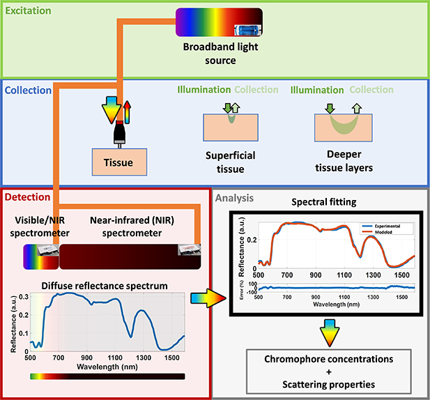
Figure 1. Schematic drawing of our DRS system and following analysis discussed in this paper. The reflected light can be collected in a wavelength range 350–1919 nm and allows the investigation of a larger variety of tissue chromophores compared to previous feasibility studies for CRC detection during colonoscopy.
Download figure:
Standard image High-resolution imageThe procedure to investigate the tissue depth probed is described in detail in [33]. Briefly the tissue depth investigated by using probes 1 and 2 was estimated through forward MC simulations of steady-state light transport in multi-layered tissues (MCML) [34] accelerated by graphics processing unit (GPU) [35, 36] using optical properties obtained from the analysis of the spectral fitting algorithm described in section 2.5. Light propagation through a semi-infinite homogeneous medium with refractive index of the outer medium (ηout) of 1, tissue refractive index (ηrel) of 1.4, anisotropy factor (g) of 0.9 was simulated. By using 10 million photon packets, we generated 5 × 5 mm light fluence maps with 10 μm of radial and depth resolution in order to compute the photon hitting density maps used to estimate the probed depth.
2.3. Optical measurement protocol
First, we collected the background and reference signals. Both these measurements were taken by placing each probe on a specialized holder designed to fix the distance between the fiber optic probes and our reflectance standard (FWS-99-01c, Avian Technologies LLC, New London, USA). Signal contamination due to backscattered light and ambient light was avoided be a closed environment with blackened walls of the holder. The background and reflectance measurements were taken with our broadband light source turned off and on, respectively. In order to avoid probe contamination, we covered our probes with polyvinyl chloride film and cleaned them with ethanol 70% after each set of measurements. All measurements of this study were performed with the same probes, which were positioned as close to 90° from the tissue surface as possible. Upon completion of the data collection, the data was safely stored for analysis. In this study, we collected a total of 1363 spectra for the small SDD probe (630 µm SDD) and 1526 for the large SDD probe (2500 µm SDD).
2.4. Data preprocessing
In order to obtain the tissue reflectance  , the intensity measurements (
 ) of each spectrometer had their background subtracted (
 ) and the resulting intensity was divided by the reference measurements
  (with background subtraction):
To merge the reflectance spectra and correct for any slight mismatch between the two spectrometers, we used the overlapping spectral range between 1090 and 1140 nm to perform an interpolation by using the weighted sum:
The resulting reflectance spectra  were used for the estimation of chromophore concentrations and scattering parameters.
2.5. Spectral fitting and extraction of biomolecule concentrations
A flowchart of the spectral fitting algorithm is shown in figure 2. Details of the steps of this algorithm can be found in the supplementary material (available online at stacks.iop.org/JPD/54/454002/mmedia). Briefly, the obtained reflectance spectra  was used to extract the tissue absorption and scattering related parameters. The absorption-based parameters included are the concentrations of blood (total hemoglobin (THb) percentage and THC), lipid (flipid), water (fwater), bile (fbile), met-hemoglobin (fmetHb), as well as oxygen saturation (StO2), and average vessel diameter R. The scattering-based parameters, on the other hand, included the reduced scattering amplitude
  , Mie scattering power bMie, and the percentage contribution of Rayleigh scattering fRay. The spectral fitting methodology is illustrated in figure 2 with a detailed description provided in the supplementary material. Briefly, the extraction was performed by using a spectral fitting based on the four types of inputs to the algorithm: the measured DR spectrum; the pure chromophore absorption spectra (
 ); the Rayleigh and Mie scattering equations yielding the scattering coefficient as a function of wavelength; as well as a look-up table (LUT) of DR (R(µa,µs)) values describing the light propagation in tissue as a function of absorption coefficients (µa) between 0.01 and 300 cm−1, and scattering coefficients (µs) between 0.1 and 1000 cm−1. The LUT was generated by using a forward MC model of light propagation into tissues, which was accelerated by GPU [35, 36]. In this model, tissue optical properties including µa and µs were used as an input to simulate the light transport inside a homogeneous semi-infinite medium and calculate the reflectance at different positions of the medium (tissue) surface. MC simulations were performed with 10 million photon packets, refractive index of the outer medium (ηout) of 1, tissue refractive index (ηrel) of 1.4, anisotropy factor (g) 0.9. The results were stored with a radial and depth resolution of 10 μm. The contribution of photons launched in the excitation fiber was accounted through convolution of the incident photon beam [37]. The modeled reflectance was obtained by integrating the reflectance values in the area of the core diameter of the collection fibers (detector area) located at the specified SDD. This integration was performed for a wide range of optical properties involving values typically found in most biological tissues [38, 39]. The result is a MC LUT associating the modeled reflectance R(µa,µs) with µa and µs values for the geometry of our fiber optic probe.
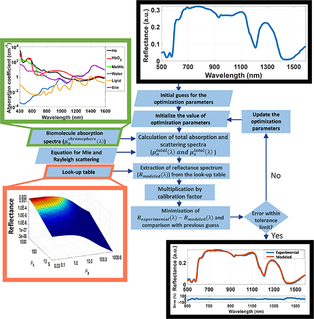
Figure 2. Flowchart of the steps of our spectral fitting algorithm.
Download figure:
Standard image High-resolution imageBy using the MC LUT, chromophore absorption spectra and scattering equations, the modeled DRS spectrum was reconstructed. First, chromophore concentrations and scattering parameters are used to obtain the tissue absorption and scattering spectra. Next, for each wavelength of these spectra, combinations of absorption and scattering coefficients were associated to values of reflectance R(µa,µs) in order to reconstruct the modeled DR spectrum  .
.  was multiplied by a calibration factor and compared to the experimental spectrum
  in a fitting algorithm. The outputs of the algorithm are a fitted DR spectrum, the values of the fitting parameters and a value for the fitting fidelity.
In the algorithm we implemented the same spectral fitting method as used by Nachabe et al [40, 41] (and is described in in more detail in the supplementary material). Validation studies of our fitting procedure were conducted in both phantoms and biological tissue samples and has been was presented elsewhere [42]. It is important to note that we refer to  as THb percentage in tissue, even though THb is a relative volume percentage of pure blood. We also emphasize that
  may contain traces of bilirubin found in blood at ranges between 5.8% and 40% in humans, especially considering that bilirubin blood serum levels can vary between 10 and 50 mg dl−1 [43] and hemoglobin blood levels vary between 121 and 172 mg dl−1 [39]. With that in mind,
  would represent the bile concentration added to a contribution of bilirubin varying between 5.8% and 40% of THb. The use of bilirubin absorption spectrum in our fitting is limited by the narrow wavelength range reported in the literature, which is not sufficient to fit a spectrum between 450 and 1590 nm.
2.6. Statistical tests
Significant statistical differences between spectral fitting parameters of normal mucosa and tumors were tested by using two-sample t-test and Wilcoxon rank sum test. To evaluate the adequate use of two-sample t-test, Anderson–Darling and Lilliefors normality tests were performed.
2.7. Classification using binary decision tree
The tissue chromophore concentrations and scattering properties obtained with our spectral fitting model were used for tissue classification in mucosa and tumor based on a binary decision tree algorithm. Our decision tree was built by using the classification and regression tree (CART) algorithm implemented with default fitctree MATLAB function. The method uses a recursive partitioning method to generate a classification tree from thresholds of the tissue parameters obtained by the spectral fitting described in section 2.5. These thresholds are selected from a training set of spectral data and applied to spectra on the test set for every iteration of cross-validation. This study used five-fold cross-validation, which consists of randomly dividing the dataset into five sets of training and test sets containing 80% and 20% of the spectra in our dataset, respectively. Each of these pairs is used to build a tissue classification model where the model is calibrated in the training set and validated on the test set. For each pair, the classification model was assessed by performance parameters involving the sensitivity, specificity, accuracy and area under the receiver operating characteristic curve (AUC) for identification tumor and mucosa tissues. The performance of the classification model was given by the mean of performance parameters among the five sets.
In order to ensure our tissue classification model was not overfitted, we reported the mean and standard deviation of the output of the 20 iterations of five-fold cross-validation with random sampling. In addition, we have used THb, R, flipid, fwater, fbile, α', fRay and bMie as relevant parameters for tissue classification. StO2, and fmetHb were not included in the model due to their variations in ex vivo settings, as it was not possible to control the blood oxygenation and conversion of Hb and HbO2 into met-Hb once blood of the specimen was exposed to air.
3. Results
3.1. Tissue chromophore concentrations and scattering properties
Our spectral fitting analysis yielded relevant absorption and scattering parameters to be used for the tissue differentiation. Based on this analysis, we selected the tissue scattering-based microstructure parameters (reduced scattering amplitude  , Mie scattering power bMie, and the percentage contribution fRay), and concentrations of blood (THb), lipid (flipid), water (fwater), bile (fbile), as well as oxygen saturation (StO2) and average vessel diameter R as relevant parameters to be monitored and discussed (figures 3 and 4). All fitted variables are described in table 2. Values of fMetHb were not considered relevant for our analysis as these values can vary due to exposure to oxidizing agents which convert Hb into metHb, even though fMetHb needed to be included in our spectral fitting in order to eliminate the metHb influence on THb, THC and StO2. Figure 3 shows a boxplot of the fitted parameters for all mucosa and tumor tissue spectra using probe 1. These plots suggest that the parameters which best discriminate mucosa and tumor tissues are THb, flipid and bMie.
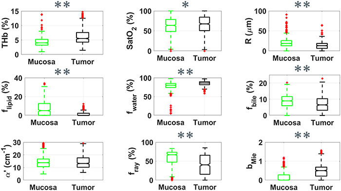
Figure 3. Boxplots of relevant parameters for differentiation between superficial tissue layers of mucosa (green, n = 728) and tumor (black, n = 635) by using probe 1. Red points represent outliers (points at more than 1.5 times the interquartile range away from the bottom or top of the box). Statistical difference for p < 0.05 is represented by * and that for p < 0.001 is represented by ** for the Wilcoxon rank sum test.
Download figure:
Standard image High-resolution image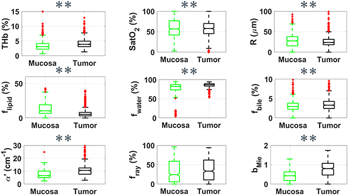
Figure 4. Boxplots of relevant parameters for differentiation between superficial tissue layers of mucosa (green, n = 804) and tumor (black, n = 722) by using probe 2. Red points represent outliers (points at more than 1.5 times the interquartile range away from the bottom or top of the box). Statistical difference for p < 0.05 is represented by * and that for p < 0.001 is represented by ** for the Wilcoxon rank sum test.
Download figure:
Standard image High-resolution imageTable 2. Biochemical and microstructural parameters of mucosa and tumor tissues investigated with the small SDD probe (superficial tissue) and the large SDD probe (deeper tissue layers).
| Biochemical/microstructural parameters | Small SDD probe (probe 1) | Large SDD probe (probe 2) | |||
|---|---|---|---|---|---|
| Abbreviation | Mucosa | Tumor | Mucosa | Tumor | |
| Total hemoglobin percentage | THb (%) | 5.0 ± 4.0 | 6.6 ± 3.9 | 3.5 ± 1.4 | 4.8 ± 1.9 |
| Total hemoglobin molar concentration | THC (μM) | 116 ± 92 | 154 ± 90 | 81 ± 33 | 111 ± 45 |
| Oxygen saturation | StO2 (%) | 64 ± 21 | 66 ± 23 | 50 ± 17 | 56 ± 18 |
| Average vessel radius (μm) | R (μm) | 25 ± 36 | 14 ± 11 | 33 ± 15 | 24 ± 13 |
| Lipid volume percent | flipid (%) | 7.7 ± 8.6 | 1.4 ± 2.2 | 14.1 ± 8.9 | 4.8 ± 3.0 |
| Water volume percent | fwater (%) | 78.5 ± 10.2 | 84.9 ± 7.2 | 79.2 ± 9.0 | 86.7 ± 4.0 |
| Bile volume percent | fbile (%) | 8.9 ± 4.5 | 7.0 ± 4.8 | 3.3 ± 1.3 | 3.7 ± 2.5 |
| Met-hemoglobin volume percent | fMetHb (%) | 1.1 ± 0.6 | 1.1 ± 0.7 | 0.2 ± 0.2 | 0.3 ± 0.5 |
| Amplitude of reduced scattering coefficient | α' (cm−1) | 14.3 ± 5.5 | 15.9 ± 10.1 | 8.2 ± 3.7 | 12.0 ± 5.6 |
| Mie scattering power | bMie | 0.2 ± 0.2 | 0.5 ± 0.3 | 0.5 ± 0.3 | 0.9 ± 0.4 |
| Rayleigh scattering fraction | fRay (%) | 56 ± 24 | 40 ± 27 | 36 ± 28 | 36 ± 28 |
Figure 4 suggests a similar behavior of chromophore concentrations and scattering properties differentiating mucosa and cancer tissues could be observed in both superficial tissue (figure 3 for probe 1) and deeper tissue layers (figure 4 for probe 2). The differentiation of parameters such as the scattering amplitude α', flipid and bMie increased by using probe 2. Yet, the trend observed for lower fRay in the tumor surface (figure 3) does not hold for deeper tissue layers in tumors.
Table 2 shows the mean and standard deviation of mucosal and cancerous biochemical and microstructural parameters extracted with our DR spectral fitting algorithm. In average, tumors had larger THb, THC, fwater, α', bMie, and smaller average vessel radius, flipid compared to normal mucosa. For probe 1, tumor tissues also exhibited lower fRay. Also, R, flipid, and bMie tend to be higher for probe 2 compared to probe 1 in both mucosa and tumor tissues, whereas all other parameters tend to be lower for probe 2. The standard deviation of THb, THC, flipid, fwater for probe 2 was lower to those of probe 1, even when considering the standard deviation relative to the mean values (coefficient of variation). The p-values of statistical tests leading to the representation of significant statistical differences in the boxplots can be found in table 3. Even though we show the result of statistical tests for t-test and Wilcoxon rank sum test, we emphasize that the distribution of spectral fitting parameters of normal mucosa and tumors are normal according to both Anderson–Darling and Lilliefors normality tests.
Table 3. P-values of t-test and Wilcoxon rank sum test for each biochemical and microstructural parameter of mucosa and tumor tissues investigated with the small probe (probe 1) and the large probe (probe 2). Statistical difference for p < 0.05 is represented by yellow background and that for p < 0.001 is represented by a green background.
| p-values of t-test | p-values of Wilcoxon rank sum test | |||
|---|---|---|---|---|
| Spectral fitting parameters | Probe 1 (s) | Probe 2 | Probe 1 | Probe 2 |
| THb (%) or THC (μM) | 1 × 10⁻⁸ | 1 × 10−45 | 8 × 10−37 | 1 × 10−45 |
| StO2 (%) | 0.140 | 1 × 10⁻¹² | 0.049 | 3 × 10⁻¹⁵ |
| R (μm) | 1 × 10⁻¹⁵ | 7 × 10⁻³⁵ | 3 × 10⁻³¹ | 2 × 10−46 |
| flipid (%) | 6 × 10−60 | 5 × 10−126 | 2 × 10−60 | 6 × 10−133 |
| fwater (%) | 6 × 10−60 | 5 × 10−126 | 1 × 10−60 | 6 × 10−133 |
| fbile (%) | 1 × 10⁻⁹ | 9 × 10⁻⁶ | 4 × 10⁻¹³ | 3 × 10⁻⁷ |
| fMetHb (%) | 0.142 | 1 × 10⁻¹¹ | 0.044 | 0.00006 |
| α' (cm−1) | 0.0006 | 1 × 10−48 | 0.930 | 6 × 10−67 |
| bMie | 1 × 10−83 | 4 × 10−101 | 1 × 10−88 | 4 × 10−93 |
| fRay (%) | 2 × 10⁻²⁹ | 0.858 | 1 × 10⁻²⁶ | 0.966 |
3.2. Tissue classification using decision trees
Classification trees were built with spectral fitting parameters of probes 1 and 2 in order to categorize tumors based on their particular ranges of chromophore concentrations and scattering properties. Figures 5(a) and (b) show the two separate branches of a decision tree with parameters leading to most of the differentiation between mucosa and tumor by using probe 1. These parameters are THb, R, flipid, fbile, α', fRay and bMie. By using the five-fold cross-validation method described previously, we achieved 81.8% ± 1.1% sensitivity, 88.2% ± 1.4% specificity, 84.8% ± 0.6% accuracy, 0.900 ± 0.007 AUC. Also, it is important to note that parameters appearing close to the top of the decision tree are the most important for tissue classification. With this in mind, the parameters which appear on the top two layers of splits for probe 1 (figures 5(a) and (b)), i.e. flipid, α', fRay and bMie, are the directly or indirectly related to tissue scattering (section 4.3).
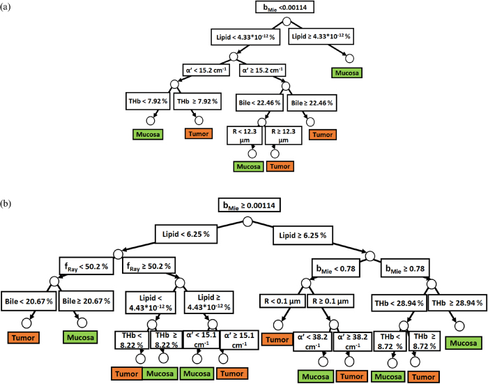
Figure 5. (a) Classification decision tree of the colorectal mucosa and tumor tissues based on parameter threshold values of probe 1 for  . (b) Classification decision tree of the colorectal mucosa and tumor tissues based on parameter threshold values of probe 1 for
  .
.
Download figure:
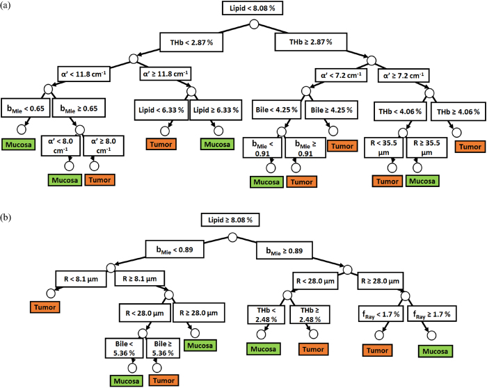
Standard image High-resolution imageSimilarly to probe 1, figures 6(a) and (b) show the two separate branches of a decision tree with parameters leading to most of the differentiation between mucosa and tumor by using probe 2. These parameters are THb, R, flipid, fbile, α', and bMie. By using five-fold cross-validation, we achieved 87.1% ± 0.6% sensitivity, 89.7% ± 1.0% specificity, 88.3% ± 0.6% accuracy, 0.911 ± 0.006 AUC. Differently from probe 1, the parameters which appear on the top two layers of splits for probe 2 (THb, R, flipid, α', and bMie) include both absorption and scattering parameters. Still, flipid, α', and bMie appear as important parameters for both probes and may be explored in future studies for endoscopic CRC detection.
Figure 6. (a) Classification decision tree of the colorectal mucosa and tumor tissues based on parameter threshold values of probe 2 for  . (b) Classification decision tree of the colorectal mucosa and tumor tissues based on parameter threshold values of probe 2 for
  .
.
Download figure:
Standard image High-resolution image
4. Discussion
4.1. Relevance of our work
The relevance of our work is highlighted by the limitations overcome with respect to prior research on CRC detection during colonoscopy using DRS. Compared to previous studies, we have collected a substantially larger (2889 DRS spectra) at the extended wavelength range between 350 and 1920 nm by using fiber optic probes with two SDDs in order to probe superficial and deeper tissue layers. By using a 630 µm SDD fiber optic probe, signals could be captured from superficial tissue at depths between 0.5 and 1 mm (>0.8 mm for most wavelengths), whereas a 2500 µm SDD probe was used to collect signals from deeper tissue layers with between 0.5 and 1.9 mm (>1.4 mm for most wavelengths) [33]. Our extraction of chromophore concentrations and scattering properties is not restricted by limitations of diffusion theory, as we use probabilistic MC models to build the LUT containing reflectance values to fit the DRS spectrum. Furthermore, our LUT covers a wider range of optical properties (scattering coefficient varying from 0.1 to 1000 cm−1 and absorption coefficient from 0.01 to 300 cm−1) and a greater resolution (7200 reflectance values) compared to past studies, to the best of our knowledge.
4.2. Analysis of DRS measurements: multivariate analysis and spectral fitting model
In general, DRS measurements can be analyzed by using either machine learning methods [18–20, 22–29] for direct tissue differentiation or by spectral fitting models to obtain information on the tissue microstructure and biochemistry [18, 19, 30–32]. Machine learning is typically employed to build models for automated tissue discrimination without interpretation of the sources of this discrimination or to identify variables contributing most to the differentiation of two or more tissue types [18–29, 44–49]. Spectral fitting is used to extract chromophore concentrations and tissue optical properties such as the absorption and reduced scattering coefficients. The accuracy of spectral fitting models is dependent on the type of light transport model used as well the scattering and absorption properties of the medium where the light propagates [31, 40, 41, 50–56].
Analytical models provide a solution to the radiative transport equation often using the diffusion approximation (typically valid when the scattering coefficient  is much higher than the absorption coefficient
  ) [52, 57–67] or use a semi-empirical solution (often valid for media with particular sets of chromophores at specific geometries), while probabilistic models often use MC simulations to compute average parameters based on the photon packet paths and processes (e.g. absorption) inside the medium [31, 40, 41, 50–56]. Even though probabilistic models are more time-consuming, they provide the most accurate solution for the present case, as diffusion models are not accurate for short SDDs and for all tissue optical properties [31, 40, 41, 50–56, 68–82]. Among probabilistic models, we can exploit forward MC simulations to generate reflectance LUTs (i.e. a reflectance database as a function of μa and μs) for producing theoretical reflectance spectra based on wavelength-dependent of optical properties (referenced at scattering spectra and chromophore absorption spectra equations described in the supplementary material).
Previous studies have used spectral fitting models based on diffusion theory [52, 57–67] and may not be accurate in estimating chromophore concentrations and scattering parameters from tissues with optical properties out of the range of validity of diffusion theory [31, 40, 41, 50–56, 68–82]. The spectral fitting model used in this study uses MC simulations for a variety of optical properties (μs ranging from 0.1 to 1000 cm−1 and μa ranging from 0.01 to 300 cm−1). Therefore, our estimation of chromophore concentrations should be more accurate than prior studies. Furthermore, we combined our determined ranges of chromophore concentrations and scattering parameters which discriminate mucosa and tumor tissues with more than 90% AUC and 84% accuracy for probes investigating tissue depth up to 1 mm (small probe) and 1.9 mm (large probe).
We combine our spectral fitting model with machine learning in order to select the thresholds of chromophore concentrations and scattering parameters for highest differentiation between mucosa and CRC tissues. The selection of these thresholds can be performed directly by using the CART algorithm with no assumptions on the data distribution (i.e. reflectance values at each wavelength). Since the decision tree resulting from CART contains the most important parameters for tissue differentiation on the top (i.e. 1st nodes) of the tree, the importance of individual parameters can be checked by the order they appear on the tree. In addition, since parameters and their thresholds can be determined by tissue differentiation, it is possible to associate them with categories of mucosa and tumors occurring in cancer patients and, in particular, to identify cases where mucosa and tumors can be differentiated from each other. Thus, the results of our analysis offer not only a way to localize tumor tissues in normal mucosa, but a way of characterizing tissue microstructure and biochemistry that may influence clinical decision-making once parameter thresholds can be assessed in future in vivo studies involving sufficient number of patients. Finally, by understanding the cancer microstructure and biochemistry, it may be possible to learn the origin of cancer and related diseases, as well as to identify cases leading to better patient prognosis.
4.3. Tissue optical scattering, HbO2, Hb, water and lipid changes in mucosa and cancerous tissues
In this study, the most important parameters for discrimination between mucosa and tumor tissues for both probes were THb, R, flipid, fbile, α', and bMie (figures 5(a), (b), 6(a) and (b)). Particularly for the small probe (probe 1), fRay was considered an important parameter for that discrimination based on reflectance of superficial tissue (figures 5(a) and (b)). As reported in previous studies, THb is expected to be higher in tumors due to the associated angiogenesis process to increase the local blood supply and support tumor growth. According to our results (tables 2 and 3 and figures 3 and 4), the investigated tumors had blood vessels with smaller average radius and slightly higher StO2 in deeper tissue layers (probe 2) compared to mucosa, which may indicate that smaller vessels are created to increase the local oxygen supply in adenocarcinomas and carcinomas. Most previous studies investigated DRS for superficial tissue layers and reported higher THb and lower StO2 in cancer tissues in relation to uninvolved mucosa [18, 19, 30–32]. By exploiting the wavelength range between 350 and 700 nm with a 550 μm SDD probe, Zonios et al [30] studied normal and cancerous tissues of 13 patients. The authors observed, respectively, THC of 13.6 ± 8.8 mg dl−1 and StO2 of 59% ± 8% for normal tissues, whereas adenomatous polyps exhibited THC of 72.0 ± 29.2 mg dl−1 and StO2 of 63% ± 10%. A higher THC and a slight increase of StO2 for potentially malignant tissues (adenomatous polyps) agrees with our results of probe 1 (630 μm SDD probe). In addition, the mucosal THC of our study (THC 9.2 ± 9.5 mg dl−1) was comparable to that of Zonios et al, while that of adenomatous polyps was about six-fold different from the THC values found in tumors of the present study (12.0 ± 8.7 mg dl−1). The difference becomes even more apparent when comparing values to findings on probe 2, where lower THC and StO2 were found (THC of 5.6 ± 2.4 mg dl−1 and StO2 of 50% ± 17% for mucosa, and THC of 7.9 ± 3.5 mg dl−1 and StO2 of 56% ± 18% for tumors, respectively). However, even lower values of THC have been found by Wang et al [31], who studied DRS of the tumors and surrounding normal tissues of 27 patients (17 with adenomatous polyps, eight with adenocarcinoma, and two with only normal tissues) in the visible wavelength range between 600 and 800 nm. By using probes with SDDs of 0.6, 1.5, 2.5, and 4 mm, Wang et al obtained mucosal THC of 59.8 ± 19.0 µM and tumor THC of 153.8 ± 38.6 µM. Even though the THC values are comparable to those of probe 2 of our study, their mucosal THC was lower while their tumor THC is higher on average (table 2). Wang et al found a much lower StO2 for tumors (26.4% ± 6.1%) compared to normal tissue (60.7% ± 7.7%), which does not agree with our study. Finally, the THC values for probe 2 of our study are comparable to results obtained by Nandy et al [83], who performed spatial frequency domain imaging to ex vivo colorectal specimens of nine patients from which 15 (eight malignant and seven normal) regions were imaged. Images were taken by using 460, 530 and 630 nm wavelengths and two spatial frequencies (0 and 1 cm−1). The authors found that THC varied between 46 and 80 μM in normal mucosa and between 57 and 118 μM in tumors.
In terms of scattering properties, tumors exhibit lower fraction of Rayleigh scattering (fRay), which may occur during cell division, when a relatively lower number of structures smaller than a wavelength exist in cells in order to create conditions for duplication of cellular structures. These structures include mitochondrion membranes (as mitochondria are under fragmentation for their equivalent distribution to daughter cells on cell division [84]) and cell membranes, replicating structures required for cell division. However, it is also important to remember that the number of mitochondria under fragmentation tends to increase during cell division in tumors. Since tumors contain cells in different stages of cell division, their tissue microstructure tends to be more heterogeneous compared to normal tissues. This heterogeneity can be observed in scattering parameters (figures 3 and 4), especially for superficial tissue (figure 3). The increase in the number of mitochondria and other organelles [85] agrees with the higher Mie scattering power (bMie) obtained in tumors, as it suggests that cancer tissues contain overall smaller-size particles and structures compared to normal tissues. Since Mie scattering is typically generated at organelle (e.g. mitochondria), nuclei, and cell scales [86], the presence of smaller structures (in average) generating Mie scattering agrees with the higher cell proliferation expected to be found in tumors [87–89].
Nandy et al [83] investigated scattering parameters by assuming an approximation of the total tissue scattering by a fitting to Mie scattering, which allows retrieving the scattering amplitude α' and the Mie scattering power bMie based on the three wavelengths investigated in their study instead of a broadband wavelength range as the present study. With this in mind, the authors reported that normal mucosa had α' between 11 and 19 cm−1, bMie between 0.78 and 1.2, whereas tumor tissue had α' between 6 and 12 cm−1, bMie between 0.2 and 0.8. While the values of α' and bMie are within the same range of those found for probe 2 in our study, their trend was exactly the opposite of our findings (lower α' and bMie for tumors compared to mucosa). Other studies have reported values of scattering coefficient at NIR wavelengths, which could be related to α', as the wavelength-dependent scattering coefficient has a much lower slope at NIR and longer wavelengths. Zeng et al [90] investigated eight cancer, one pre-malignant polyp, and five normal mucosa regions of nine patients by using a swept source-optical coherence tomography (SS-OCT) system. This system used 1310 nm as the center wavelength and had 110 nm for the full width half maximum bandwidth. In their study, cancerous specimens exhibited mean scattering coefficients (per image) ranging from 4.54 to 9.17 mm−1, whereas those of normal tissues ranged from 2.50 to 8.21 mm−1. The slightly higher scattering coefficients found in tumors agrees with the results of our study, as α' was higher for cancer tissues (table 2). On the other hand, higher scattering coefficient values disagree with results reported by Zhang et al [91], who used a spectral-domain OCT system with center wavelength at 850 nm and spectral bandwidth of 40 nm to study 16 cases of malignant and normal colorectal tissues. The authors found that the scattering coefficient of 1.41 ± 0.18 mm−1 for malignant tissues (variation between 0.25 and 2.69 mm−1) and 2.29 ± 0.32 mm−1 for normal tissues (values ranging from 1.09 to 5.41 mm−1). Although scattering parameters have different trends among studies, it is important to consider that the wavelength range has a large influence on the probed depth and tissue layers investigated. Thus, microstructural parameters will differ, especially given the heterogeneity of tumor tissues. However, the range of α' and bMie obtained in this study (table 2 and figures 3 and 4) was still in a range, which is comparable to previous studies. Factors contributing to the difference between mucosa and cancer tissues were described by Backman and Roy [16] in terms of early increase in blood supply as well as nanostructural and microstructural changes such as alterations in the collagen fiber crosslinking, cytoskeleton, chromatin structure.
An indirectly related parameter with scattering is the lipid concentration, as lipid is present in structures which generate Rayleigh scattering such as membranes and lipid droplets [92]. Then, a lower flipid in tumors (tables 2 and 3 and figures 3 and 4) may mean less membranes and lipid droplets are present in the targeted cells/tissues, which leads to lower fRay (table 2). In both probes 1 and 2, the lipid content is lower in tumors (tables 2 and 3), which agrees with previous cancer studies [93, 94]. In a Raman spectroscopy study, Bergholt et al [93] found that colorectal tumors (adenomas and adenocarcinomas) had lower lipid concentration in relation to hyperplastic polyps and higher water content compared to normal tissues. A decrease in lipid concentration in cancer tissues is further confirmed with magnetic resonance spectroscopy in breast cancer [94]. Similar studies showed that tumors contain higher water-to-lipid ratio [95–99], which also agrees with the results of this study (table 2). Therefore, lipid and water content can be used individually or in combined parameters for cancer detection.
Finally, a combination of the parameters THb, R, flipid, fbile, α', bMie, fRay was sufficient to provide classify normal mucosa and cancer tissues with 84.8% ± 0.6% and 88.3% ± 0.6% accuracy with probes 1 and 2, respectively (figures 5(a), (b), 6(a) and (b)). The parameter selection for classification of the decision trees (figures 5(a), (b), 6(a) and (b)) described nine subtypes of mucosa and tumors for probe 1 as well as ten subtypes of mucosa and tumors for probe 2. The number of tissue types shows that tissues interrogated with probe 2 tend to more heterogeneous compared to those interrogated with probe 1 (figures 5(a), (b), 6(a) and (b)). Even though the division into more tissue subtypes was expected from probing deeper tissue layers, it is important to note that the classification performed with probe 2 used less parameters (THb, R, flipid, fbile, α', bMie) compared to probe 1 (THb, R, flipid, fbile, α', bMie, fRay) and still obtained a higher tissue classification performance.
4.4. Considerations on biomolecular concentrations and probed depth for CRC detection
In our previous work [33], we showed that the probed depth for probe 1 ranges from 0.5 to 1 mm (0.8 to 0.9 mm for most wavelengths between 430 and 1590 nm), whereas that of probe 2 mostly between 0.5 and 1.9 mm (higher than 1.4 mm for most wavelengths between 430 and 1590 nm). Even though it is possible to quantify the probed depth, specifying which tissue layers are being probed in the colorectal wall still remains a challenge. A typical thickness of the total wall is about 2 mm, which may also be changed by a number of factors [100]. Individual thicknesses of the tissue layers may have a wide range of thicknesses. According to Castro-Poças et al, mucosa layers can vary from 0.3 to 1.2 mm, submucosa can vary between 0.2 and 1.8 mm and muscularis propria can vary from 0.3 to 2.4 mm [100]. This variance may contribute to the heterogeneity of the biochemical and microstructural parameters obtained in the present study (table 2). However, when comparing these parameters per probed depth, THb, THC, flipid, fwater extracted from DRS spectra of probe 2 exhibited a relatively lower coefficient of variation compared to those of probe 1. This result suggests that probing more tissue layers with probe 2 did not generate more inhomogeneity on absorption parameters such as THb, lipid and water concentrations. It is unclear how probing deeper tissue layers affects other parameters and it is expected that multilayered tissue structures influence the scattering parameters reported in this study.
In addition, our results indicate that deeper tissue layers of mucosa and tumor tend to have higher average vessel radius (R), lipid concentration (flipid), and Mie scattering power (bMie), whereas all other parameters tend to be lower for probe 2 (table 2 and figures 3 and 4). For tumors, a slightly higher R in deeper tissue layers may happen due to probing relatively less thin blood vessels (compared to the total number of vessels in the probed volume) created in the tumor surface during angiogenesis. A similar conclusion may be drawn from lower THb and THC (table 2 and figures 3 and 4), as most of the blood volume would be present on the superficial tissue layers. Since less blood vessels occur in deeper tumor layers, it would be expected a slower cell division, larger-sized cells, and less fragmented mitochondria. These three expected features lead to less refractive index mismatches, which agrees with our decreased scattering amplitude α'. Assuming Mie scattering is mostly generated by mitochondria [86], a lower number of mitochondria (larger size) would mean lower bMie, as per our results. Also, lower cell division rates mean less fragmented mitochondria, which generates less refractive index mismatches due to water-membranes transitions and thus leads to lower fRay. Finally, fwater was expected to be lower in the tissue surface due to dehydration caused during our ex vivo measurements. On the other hand, our procedure of keeping the tissue hydrated with a damp cloth from times to times during our measurements may have affected the water content extracted with our spectral fitting algorithm.
4.5. Validity and limitations of our study
Our study has several limitations due to variations caused in ex vivo tissues and contact measurements. First, the interrogated cancer tissues were from diverse stages with predominance of advance stage tumors (pT2 and above). The measured tumor sites were selected based on the palpation and naked eye determination by experienced surgeons who demarcated the tumor region, although all these regions were confirmed subsequently with histology. It is important to note that this determination does not decrease the validity of our dataset and biochemical/microstructural analysis, as our dataset is larger compared to previous studies in the field (1363 spectra for probe 1 and 1526 for probe 2) and contains DRS spectra with variations due to parameters discussed in this section. With this in mind, early-stage cancer changes are expected to occur over the same tissue biomolecules and microstructure parameters but with lower magnitude in relation to advanced cancer.
Since our measurements were performed in ex vivo colorectal specimens, the blood oxygenation was not controlled during our data collection. However, we confirmed there was no significant variations on average Hb and HbO2 in mucosa and tumor regions in a pilot ex vivo observation of the DRS signal in three patients. Our observation was limited by seven mucosa and seven tumor sites during the 1st 15 min of our measurements (data not shown). We are also aware that THb and StO2 may increase and fwater may decrease in ex vivo tissues compared to in vivo, as described by Baltussen et al [101] in a previous study investigating different types of colorectal tissues (fat, tumor, and healthy colorectal wall). It is also important to note that, although the authors used the same optical technique (DRS) to draw those conclusions, their probe has a different SDD (1.29 mm center-to-center distance) compared to those of this study and their spectral fitting model uses diffusion theory approximation to estimate THb, StO2 and fwater. In addition, the behavior of StO2 is still not well understood, as previously reported studies disagree on their StO2 trend on ex vivo tissues. While Baltussen et al reported an increased StO2 in ex vivo tissues within 1 h after resection in relation to in vivo tissues, Salomatina et al [102] reported a decrease in StO2 in mouse ear tissues 5–10 min after excision (ex vivo) of tissue and after 24 and 72 h of storage. Even though StO2 varies, it was not considered as a relevant parameter in the classification of our decision tree. Also, we attempted to reduce tissue dehydration as much as possible by keeping the tissue moisture with a water wet wipe once every seven spectral measurements in average during the measurements. We attempted to not overhydrate tissues as they were wiped by not using an overly wet wipe. As illustrated by our results, only a small deviation on water content was found in tumor measurements, which can be mainly attributed to the tissue heterogeneity expected from cancer. Furthermore, if overhydration due to uncontrolled wiping (relatively 'random' event) had influenced our measurements, higher standard deviations in water concentration should have been associated with higher water-concentration measurements (i.e. tumor measurements), which is not what we observed.
We acknowledge that probe contact pressure and sufficient optical contact with interrogated tissues may be challenging to accomplish during in vivo endoscopy. With this in mind, a reduced sensitivity to optical contact and probe positioning is expected in our probe 2 due to its larger SDD, which may be related to higher measurement repeatability and less standard deviation present in some parameters of this probe. However, larger SDDs also means larger probed volume, which may cause more variations upon probe contact pressure if this pressure allows collecting the signal from heterogeneities of deeper tissue (e.g. interface between tissue layers). This type of variation was previously reported [103] and needs to be taken into account in order to correct DRS spectra. One should also note that the incorporation of large SDD probes is feasible in colonoscope channels, as long as the probe fits the diameter of the instrument channel (typically 2.8–4.2 mm [104, 105]).
Finally, not including non-cancer pathology in our study may change the classification performance of our CART model. With this in mind, future studies will include data on non-cancer pathology. On the other hand, the lack of non-cancer pathology does not affect our tissue biochemical/microstructural parameters. Therefore, comparison of these parameters with other studies is valid, especially considering our dataset includes a robust sampling of intra- and inter-patient variations (1363 + 1526 spectra of 47 patients) in both superficial and deeper tissue layers.
5. Conclusions
In this study, we assessed the most important microstructural and biochemical parameters for endoscopic CRC detection through broadband DRS as well as the thresholds of these parameters for differentiation between mucosa and tumors. These parameters were THb, R, flipid, fbile, α', bMie, fRay, which were used to classify tissues based on decision trees for interrogating superficial (probe 1) and deeper (probe 2) tissue layers. When considering the most important parameters for CRC detection, emphasis can be given to flipid, α', and bMie, as these parameters appeared on the top of decision trees of botsh probes. Tissue classification with more than 90% AUC was achieved with both probes, with classification using probe 1 leading to 87.1% ± 0.6% sensitivity, 89.7% ± 1.0% specificity, 88.3% ± 0.6% accuracy, 0.915 ± 0.006 AUC, whereas that of probe 2 achieved 81.8% ± 1.1% sensitivity, 88.2% ± 1.4% specificity, 84.8% ± 0.6% accuracy, 0.900 ± 0.007 AUC. Therefore, the extracted parameters are relevant for cancer identification in the colorectal lumen. Furthermore, we solved the limitations of previous studies in terms of the quantification of independent tissue biochemical and microstructural parameters on superficial and deeper tissue layers without restrictions of diffusion theory and at an extended wavelength range for DRS.
To the best of our knowledge, this is the first study to evaluate the potential tissue biomolecule concentrations and scattering properties in superficial and deeper tissue layers for CRC detection in the luminal wall. Our study was conducted in ex vivo tissues and shows a proof-of-concept of probing tissue biochemistry and microstructure to be extended to in vivo interrogation during endoscopy. In a practical perspective, this study could potentially be used to develop a probe for CRC detection as well as indicate important tissue parameters for clinical decision-making during colonoscopy. The integration of this capability into a flexible fiberoptic probe which could be passed down a scope working channel could identify more subtle mucosal abnormalities such as sessile serrated polyps as well as obviate the need for multiple biopsies or polypectomies of normal mucosa. In the long-term, identifying tissue microstructure and biochemistry related to CRC could help understanding its origin and natural history, as further tissue biochemical information can be extracted non-invasively and in real-time and possibly complement biochemical analysis that require time-consuming laboratory procedures. Our study provided a first-step on this type of analysis by recognizing categories of CRC and surrounding mucosa which can be found in cancer patients as well as the thresholds of tissue chromophores and scattering parameters characterizing each type of tissue. These parameters could potentially be combined with other analysis to help clinical decision-making and to improve patient prognosis.
Acknowledgments
We acknowledge Eduardo Moriyama for the advice and logistics of the project associated with this manuscript, Shree Krishnamoorthy for the discussions on the same project, Haiyang Li for the design and assembly of the holder of the DRS system, Noel Lynch and Andrew McGuire for specimen retrieval of patients of this study and all the logistics related to it, Vivienne Curran, Aoife Foyle, Una McAuliffe, Evelyn Flanagan, Shauni Fitzgerald, and Edmund Manning for all the logistics of clinical procedures, research ethics documents, and search for patient information. Shauni Fitzgerald and Edmund Manning were funded by the Mercy Foundation. This study received financial support from Science Foundation Ireland (SFI): Grant ID SFI/15/RP/2828.
Data availability statement
The data that support the findings of this study are available upon reasonable request from the authors.
Author contributions
M S N Conceptualization, Methodology, Software, Validation, Formal analysis, Investigation, Resources, Data Curation, Writing—Original Draft, Writing—Review and Editing, Visualization, Supervision, Project administration, M R Conceptualization, Methodology, Software, Validation, Formal analysis, J e.g. Conceptualization, Methodology, Software, Validation, S M Investigation, Data Curation, M. Investigation, Data Curation, Software, H L Methodology, Investigation, S K Investigation, Resources, Data Curation, M O R Conceptualization, Methodology, Validation, Investigation, Resources, Data Curation, Writing—Review and Editing, Supervision, Project administration, Funding Acquisition, S A E Conceptualization, Methodology, Resources, Software, Validation, Formal analysis, Investigation, Data Curation, Writing—Original Draft, Writing—Review and Editing, Visualization, Supervision, Project administration, Funding Acquisition.
Conflict of interest
The authors declare no conflicts of interest.