

Abstract
We study the effects of absorption in the medium on synthetic aperture imaging. We model absorption using the loss tangent, which is the imaginary part of the relative dielectric permittivity, and study two cases: (i) the loss tangent is known and (ii) the loss tangent is unknown. When the loss tangent is known and used in Kirchhoff migration (KM), we find that images of targets are range-shifted by approximately a central wavelength so that their predicted locations are closer to the synthetic aperture than they actually are. In contrast, we find that when the medium is unknown, the KM image does not exhibit this range-shift. Hence, we determine that it is better to not make use of any knowledge of the absorption when imaging. Using a recently developed transformation of KM images, which we call reciprocal-KM (rKM), we achieve tunably high-resolution images of targets through adjusting the value of a user-defined parameter ε. When rKM is applied to an imaging region containing two targets, we find that their predicted locations shift, especially in range, but within a fraction of central wavelength of their true locations.
Export citation and abstract BibTeX RIS
1. Introduction
We consider the problem of imaging scatterers in a lossy medium. Motivated by applications of ground penetrating radar [1], we examine a synthetic aperture imaging configuration that uses only a single transducer. The data are scattered fields recorded over the synthetic aperture formed as the transducer moves along a trajectory, emits pulses, and records the response of the medium. The antenna design and optimization as well as the noise pattern and radar pulse play an important role in the applications [2, 3]. As is well known, the dielectric properties of soil are affected by the moisture in it which, in turn, affects the attenuation and dispersion of the waves [4]. We focus our attention here on attenuation and study its effects on imaging the location of small targets embedded in lossy media.
Although our motivating application is ground penetrating radar, attenuation plays an important role in several other imaging applications such as tomographic optoacoustic imaging [5] and geophysical imaging [6]. It is known that acoustic and seismic wave attenuation [7] needs to be accounted for in time reversal and imaging applications [8, 9].
Several approaches have been proposed for imaging with synthetic aperture data. The simplest and most popular one is Kirchhoff Migration (KM) [10, 11]. In KM one back-propagates the received echoes into every point in the imaging window (IW) of interest. The echoes coherently interfere and produce a peak at points where scatterers are located while they average to zero at the background. By plotting the results of this back-propagation over a mesh of the IW, we form an image with peaks located at or very near the locations where scatterers reside. The resolution of the image is often quantified using the point spread function, which is the reconstructed image for a point scatterer. The resolution depends on the size of the synthetic aperture, a, and the bandwidth, B, of the emitted pulse. In a non-attenuating medium the cross-range resolution (in the direction parallel to the synthetic aperture) is  with λ the central wavelength and L the distance of propagation and the range resolution is
  with c the speed of the waves.
Accounting for attenuation in the medium, we carry out a resolution analysis for KM imaging. We show that cross-range resolution is not significantly affected by attenuation, but range resolution is. The image becomes more diffuse (less focused) as  increases with β denoting the loss tangent, i.e. the imaginary part of the relative dielectric permittivity. There is also a shift that is introduced in the image where the scatterer appears at a range that is closer to the synthetic aperture than it really is. Surprisingly reconstructions are better when attenuation is completely ignored in image formation. This result implies that even if we know the attenuation in the medium, we should not use that knowledge during the back-propagation step in KM. Intuitively that can be understood as follows. By back-propagating in an attenuating medium, waves undergo the loss twice. As argued Devaney [8], when imaging in attenuating media, one may chose to amplify the scattered wave by back-propagating in a medium that acts like a pump. However, doing this will lead to instabilities when the measurements are corrupted by noise as is the case for near-field imaging when exponentially small evanescent components of the waves are used for imaging [12].
Following our recent work on the modification to the multiple signal classification method (MUSIC) for SAR imaging [13] we introduced in [14] a modification to the classical KM that allows for high resolution imaging with noisy data. There are two key elements in the modification of MUSIC: (i) the use of both the noise and the signal subspaces of the data and (ii) the introduction of a user-defined tuning parameter, which we call ε. This parameter can be made arbitrarily small and thus allows for tunable high-resolution imaging. However, just like MUSIC, this modified method, which we call ε-MUSIC, is limited to data with sufficiently high signal-to-noise ratios (SNRs) so that there is a clear separation between the signal and the noise subspaces. By identifying the elementary mechanism leading to tunable resolution, we introduced an elementary transformation of classical KM image [14] and have achieved tunably high resolution images.
Here, we use this modified KM to obtain high-resolution images in lossy media. This imaging method is a Möbius-type transformation of the classical KM imaging functional that depends on the user-defined parameter, ε. We call this transformation the reciprocal-KM (rKM) imaging functional. It leads to the superior resolution estimates of  in cross-range and
  in range. Because ε is a user-defined parameter, these resolution estimates can be made arbitrarily small. The key idea in rKM is that it sharpens a peak of a normalized KM image. Consequently, one needs to distinguish different scatterers using KM first. In other words, rKM can indeed be used to obtain high resolution images of multiple targets, but these targets need to be sufficiently far apart so as to be resolved by the classical KM image. In contrast to MUSIC, there is no singular value decomposition and no need to separate the signal from the noise subspaces in rKM. Thus this method can be used in low SNR scenarios. It is also very easy to compute and requires no additional calculations beyond the classical KM image.
The remainder of the paper is as follows. In section 2 we present the description of the imaging problem, our model for the data, and the classical KM imaging functional. In section 3 we carry out the resolution analysis in a known lossy medium. In section 4 we consider the case in which attenuation is not known so back-propagation is done in a non-attenuating medium. In both cases numerical results are presented that are in agreement with our theoretical results. In section 5 the rKM imaging functional is introduced. Numerical results illustrating the resolution estimates and high-resolution images are obtained for single and multiple scatterers embedded in lossy media. The results remain essentially the same for data with low SNR indicating the robustness of the method to noise. We finish with our conclusions in section 6.
2. Problem description
We describe the synthetic aperture imaging problem that we consider here. A single transducer is used to probe an IW containing scattering targets. This transducer emits signals and records the subsequent responses at each of the known locations:
x
r
for  , which form a synthetic aperture of size a. The collection of individual experiments in which the transducer emits a signal and records measurements of scattered fields at each spatial location
x
r
is the data for this problem. The objective for this imaging problem is to recover locations of targets, denoted by
, which form a synthetic aperture of size a. The collection of individual experiments in which the transducer emits a signal and records measurements of scattered fields at each spatial location
x
r
is the data for this problem. The objective for this imaging problem is to recover locations of targets, denoted by  contained in the IW from this set of data.
A sketch of this synthetic aperture imaging problem appears in figure 1. We characterize this imaging system by the length L, which is the distance from the center of the synthetic aperture to the center of the IW, and the system bandwidth B. Each signal emitted by the transducer uses frequencies  for
for  where ω0 denotes the central frequency. Measurements of scattered fields are also taken over these frequencies.

Figure 1. Sketch of the synthetic aperture imaging system we consider here. A single transducer emits signals and records subsequent responses at known locations:
x
r
for  , which form a synthetic aperture of size a. The length L characterizes the distance from the center of the synthetic aperture to targets located at
  in the imaging window.
Download figure:
Standard image High-resolution image2.1. Parameter values
In the numerical simulations we use to test and validate the theory presented here, we use parameter values based on ground penetrating radar applications for detecting unexploded ordnance. We consider a coordinate system whose origin is centered on the synthetic aperture (see figure 1). The locations of the spatial measurements are  with
with  for
for  , where
  and a = 150 cm. We use
  frequencies sampling the frequency range, 125–250 MHz. In wet sandy soil the wavespeed is
  m s−1, so that the corresponding wavelengths for this frequency range are 30–60 cm [15]. We set the characteristic length to be L = 200 cm. The IW is the region corresponding to
  and
and  in this coordinate system.
2.2. Measurements
Suppose there are M point targets in the IW at locations  for
for  . Assuming that the transducer emits a spherical wave with unit amplitude, the data recorded at location
x
r
at frequency ωl
is given by
. Assuming that the transducer emits a spherical wave with unit amplitude, the data recorded at location
x
r
at frequency ωl
is given by
with ρj
for  denoting the reflectivities of the targets and

denoting the Green's function for the medium (see [1]). Here c is the wave speed and  is the loss tangent which is the imaginary part of the relative dielectric constant. We use this parameter to model absorption in a lossy medium. When β = 0, there is no absorption in the medium. Larger values of β correspond to stronger absorption in the medium. A typical value for the attenuation in wet sandy soil is 1.5 dB per meter (measured at 100 MHz frequency [16]) which corresponds to β = 0.08.
2.3. KM
In what follows, we use KM to recover the location of the targets. The KM imaging functional is formed by backpropagating the data in the medium, i.e. the image at point y is computed as

Here, we call  the illumination function. We specify illumination functions below depending on our knowledge of the medium. To obtain an image we evaluate
  on a mesh discretizing the IW.
In a homogeneous, lossless medium, the resolution of the KM imaging functional given in (3) is  in range and
  in cross-range with λ denoting the central wavelength. Using the parameter values specified above, we have ∼30 cm resolution in cross-range and ∼45 cm resolution in range. We use these resolution estimates as a benchmark for the results we obtain below for lossy media.
3. Imaging in a known lossy medium
When the medium is known, β is known. Thus, we use

with

for the illumination function in (3). We first compute a resolution analysis for a single point target. Then we present and discuss numerical results that validate this theory.
3.1. Resolution analysis
To carry out the resolution analysis for KM in a lossy medium that is known, we consider the problem of imaging a single point target. This point target is located at  . Assuming that the reflectivity of the target is ρ = 1, we have the following model for our measurements,

Assuming that the measurements over frequency and space are dense enough, we replace the discrete sums in (3) by integrals so that,

Substituting (2) into (6) and substituting that result into (7), we obtain

where we used the Taylor expansion about β = 0 to obtain the approximation,

Assuming that we are in the far field, the denominator in (8) does not affect the resolution and can be replaced by  . Focusing on a small neighborhood about
  and assuming the array aperture is small compared to the distance L, we use the paraxial approximation in the phase, i.e.
leading to
Since the term  appears in the phase of (8) we have kept terms up to
  . In contrast the term
  appears in the exponential decay of (8), so we have only kept terms up to O(1).
To obtain an estimate for the resolution in range, we substitute the paraxial approximations above into (8), evaluate that result on  , and obtain

This expression tells us that IKM behaves like a  function in range,

For β = 0, we have  and
and  . It follows that this expression reduces to the well known result from which we determine that range resolution is
  . For β > 0, the term involving
  may be large enough to affect the image significantly as z varies.
We obtain an estimate for the resolution in the cross-range direction by evaluating (8) on  which yields


where we have substituted  . When β = 0 this expression reduces to the well known result from which we determine that cross-range resolution is
  . In contrast to what we have found for the range, the term involving β2 will not affect the image significantly because it does not depend on x or z and hence only scales the overall result.
3.2. Numerical results
We now present images produced using KM as defined in (4) for a point target located at  with
with  cm and
  cm. Recall that L = 200 cm here. In figure 2 we plot
  normalized by its maximum value for (a) β = 0.04, (b) β = 0.08, and (c) β = 0.10 in a region centered about the target location, which is plotted as a red '+' in each of the figures.
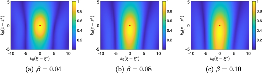
Figure 2. Image produced by KM for a known, lossy medium with (a) β = 0.04, (b) β = 0.08, and (c) β = 0.10.
Download figure:
Standard image High-resolution imageThese images show that the value of β greatly affects the image, especially with respect to z, the range coordinate. These results show that the peak of the image produced using KM 'shifts below' from the true target location. Because of absorption in the medium, these KM images are producing errors in which targets are predicted to be closer in range to the synthetic aperture than they actually are. We have seen this phenomenon before with diffuse optical imaging [17]. Thus, this imaging method produces errors in identifying and recovering target locations.
In figure 3 we show slices of the images shown in figure 2 on (a)  to show the range dependence and (b)
  to show the cross-range dependence. The solid curves are
  normalized by its maximum value. The dashed curves are evaluations of the paraxial approximations
with  , and
, and

 , for figures 3(a) and (b), respectively. We use these approximations rather than those that use the integration approximation because
  and
and  are relatively small. These analytical approximations capture the behavior of the images in range and cross-range. Specifically, they show that the peak of the image shifts with β and broadens in range, but remains relatively unchanged in cross-range. However, the shift in range over these values of β are within a central wavelength away from the true range value. To illustrate the effect of the depth L in the reconstructions we show in figures 3(c) and (d) results obtained for L = 300 cm. We observe that the shift in range increases with depth while resolution in cross-range also deteriorates as predicted by (13) as it is proportional to
  .
.

Figure 3. (a) Range and (b) cross-range slices of the KM image for a known, lossy medium (solid curves) with comparisons using the analytical approximation (dashed curves) for different values of the loss tangent β with L = 200 cm. Plots (c) and (d) show the same as (a) and (b), but with L = 300 cm.
Download figure:
Standard image High-resolution imageUsing KM to image targets in a lossy medium that is known is problematic. Specifically, the numerical results show that images suffer from a loss in range resolution. More importantly, they show that the peak of the image which is used to identify and locate targets is shifted in range by approximately one central wavelength. Hence, one cannot reliably use this method to obtain precise estimates for a target's location.
4. Imaging in an unknown lossy medium
In the preceding section, we have shown that absorption in the medium modeled by the loss tangent β degrades the utility of the images. However, for many practical problems, the exact value of β is unknown since conditions that affect its value such as the composition of materials contained in the medium, moisture, etc are unknown. For that case, we consider instead using the illumination function,

with Φ0 defined in (5) with β = 0. In what follows, we give a resolution analysis for this illumination function and show numerical results.
4.1. Resolution analysis
Using the same notation and approach we used for the previous case, we find that

Proceeding as we have done in section 3.1, we find that

and

A key difference in these results is that in (16), the terms with  have no dependence on the search coordinates x or z. Consequently, this term will affect the scaling, but not the overall shape of the image. We anticipate that images formed this way will not exhibit the range-shift in the image peak observed in the previous case.
4.2. Numerical results
We now present images produced using KM as defined in (14) for a point target located at  cm with
  cm and
  cm. Recall that L = 200 cm. In figure 4 we plot
  normalized by its maximum value for (a) β = 0.04, (b) β = 0.08, and (c) β = 0.10 in a region centered about the target location, which is plotted as a red '+' in each of the figures.

Figure 4. Image produced by KM for an unknown, lossy medium with (a) β = 0.04, (b) β = 0.08, and (c) β = 0.10.
Download figure:
Standard image High-resolution imageIn contrast to the results shown in figure 2, these images show that the value of β does not affect the image significantly in either range or cross-range. We do observe some broadening of the image peak as β increases. However, there is no significant shifting of the peak location, so this method reliably locates targets.
In figure 5 we show slices of the images shown in figure 4 on (a)  to show the range dependence and (b)
  to show the cross-range dependence. The solid curves are
  normalized by its maximum value. The dashed curves are evaluations of the following paraxial approximations,

with  , and
, and
with  , for figures 5(a) and (b), respectively. These analytical approximation capture the behavior of the images in range and cross-range. Specifically, they show that the images broaden only slightly with β.
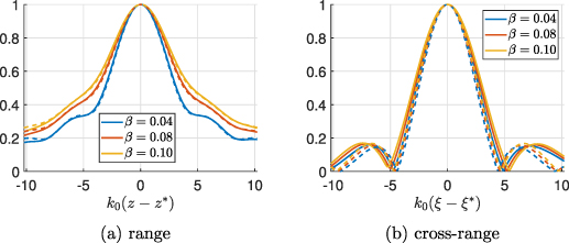
Figure 5. (a) Range and (b) cross-range slices of the KM image for a known, lossy medium (solid curves) with comparisons using the analytical approximation (dashed curves) for different values of the loss tangent β.
Download figure:
Standard image High-resolution imageSurprisingly, we have found that using KM to image targets in a lossy medium that is unknown to be better than imaging when the lossy medium is known. Although the images suffer in resolution with absorption, there is no range-shift in the peak of the images. Therefore, this method can be used to obtain precise estimates for target locations.
5. High-resolution imaging using rKM
We have recently developed a simple transformation of the KM image that produces a tunably high-resolution image. To explain the idea, let us consider the function  . This function attains its maximum value of 1 on x = 0. Its full-width/half-maximum (FWHM) is O(a). The function
is a simple Möbius-type transformation of  involving the parameter ε. This function also attains its maximum value of 1 on x = 0. However, it can be easily shown that its FWHM is
  .
.
Motivated by this example, we introduce the following rKM imaging functional,

Here ε is a user-defined parameter that can be adjusted to tune the resolution which will be  in range and
  in cross-range.
We have found that imaging without knowledge of the medium yields better results than when we use knowledge of the medium. In figure 6(a) we show again the image produced using KM as defined in (14) with β = 0.08. When we transform that KM image in figure 4(b) using (18) with ε = 0.01, we obtain the result in figure 6(b). Transforming the KM imaging using rKM produces a significantly higher resolution image.
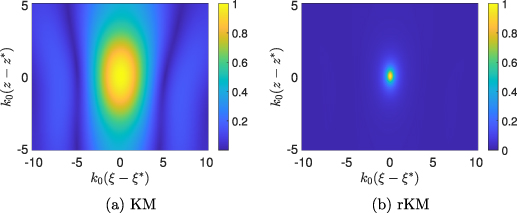
Figure 6. Comparison of the images produced using (a) KM as defined in (14) for β = 0.08 and (b) rKM applied to that image with ε = 0.01.
Download figure:
Standard image High-resolution imageTo verify that the resolution estimates for rKM scale with  , we evaluate (18) on the image produced using KM with (14) with β = 0.08 for varying values of ε. We then numerically determine the FWHM of those resulting images in both range
  and cross-range
  . Those results scaled by
  are shown in figure 7 as blue circles for range and red squares for cross-range. For reference, we have plotted a black dashed curve that is
  . The solid blue and red curves show the least-squares linear fit to these data. The results of these least-squares fits are
  and
and  which validate the
  behavior of the resolution of these images.
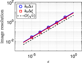
Figure 7. Numerically computed FWHM of images produced using rKM with varying values of ε on the KM image using (14) for β = 0.08. The blue circle and red square symbols plot the range  and cross-range (
 ) FWHM data, respectively. The blue and red solid curves plot the least-squares fits to lines through these data. The black dashed curve gives a reference for
  behavior.
Download figure:
Standard image High-resolution imageWe now apply rKM in an IW where there are two targets. A key point with (18) is that it uses a normalized KM image and sharpens the image about its peak value of 1. When there are two or more targets, the normalized KM image may only have one peak normalized to 1. The other peaks corresponding to other targets may be smaller. To be able to obtain high-resolution images of each of the peaks, we isolate individual peaks in subregions of the IW in the KM image. Each of these KM images in these subregions may be normalized by their local peak values and therefore (18) can be applied successfully.
In figure 8(a) we show the KM produced in a lossy medium with β = 0.04 and L = 200 cm with two targets with different ranges, but the same cross-range. Target 1 is located at  with
with  cm and
  cm. Target 2 is located at
  with
with  cm and
  cm. These target locations are plotted in figure 8(a) as red '+' symbols. White dotted rectangles indicate the subregions of the IW used to isolate the peaks of this KM image. We plot the rKM images using ε = 0.01 for target 1 in figure 8(b) and for target 2 in figure 8(c) in their respective subregions.

Figure 8. (a) Image produced by KM for an unknown, lossy medium with two targets. (b) Image produced by rKM with ε = 0.01 in a region about the location of target 1. (c) Image produced by rKM with ε = 0.01 about the location of target 2.
Download figure:
Standard image High-resolution imageThe KM image shown in figure 8(a) shows a stronger peak for target 2, whose range location is less than that for target 1, so it is closer to the synthetic aperture. Additionally, we observe that the range location of the peak in the KM image for target 1 is larger than the true value. In contrast, the range location of the peak in the KM for target 2 is smaller than the true value. When we plot the rKM images in the subregions of the IW, we see that the high-resolution peaks are shifted in range from the true locations of the targets. However, these shifts in range are much smaller than the central wavelength (they are of the order of  ).
).
In figure 9(a) we show the KM produced in a lossy medium with β = 0.04 and L = 200 cm with two targets with the same ranges, but different cross-ranges. Target 1 is located at  with
with  cm and
  cm. Target 2 is located at
  with
with  cm and
  cm. These target locations are plotted in figure 9(a) as red '+' symbols. White dotted rectangles indicate the subregions of the IW used to isolate the peaks of this KM image. We plot the rKM images using ε = 0.01 for target 1 in figure 9(b) and for target 2 in figure 9(c) in their respective subregions.
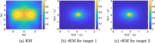
Figure 9. (a) Image produced by KM for an unknown, lossy medium with two targets. (b) Image produced by rKM with ε = 0.01 in a subregion about the location of target 1. (c) Image produced by rKM with ε = 0.01 in a subregion about the location of target 2.
Download figure:
Standard image High-resolution imageThe rKM images shown in figures 9(b) and (c) form peaks closer to the true target locations in comparison to the images shown in figures 8(b) and (c). However, there are shifts in the cross-range locations of the targets for these two targets. These shifts are much smaller than the ones observed for range-separated targets.
Thus far we have not added noise to the measurements. One advantageous feature of KM imaging is that it works well even with measurements corrupted by additive noise.
To add noise to the data we proceed as follows. Considering the noise free data  for
for  and
and  as a
as a  matrix, D, whose elements are given by (1) we add to it a noise matrix,
  with zero mean uncorrelated Gaussian distributed entries and variance
  , i.e.
  . Here the average power received per transducer location and frequency is given by
The expected power of the noise W over all transducer locations and frequencies is
with  denoting the Frobenius matrix norm. As the total power of the signal received over all transducer locations and frequencies is
  , the SNR in dB defined as
  has a mean of
  . In figures 10 and 11 we show images formed by KM for the same target configurations as figures 8 and 9, respectively, but with noise added to the measurements. For figure 10,
  dB and for figure 11,
  dB. In comparison to figures 8 and 9, we find that the images in figures 10 and 11 are nearly identical. The images formed using rKM show that the high-resolution peaks are also shifted from the true target locations but the shift is much smaller than the central wavelength. The shifts of these peaks are slightly different from those in the noiseless images. However, the overall image characteristics are the same. Hence, we determine that this imaging method is effective for low-SNR settings.
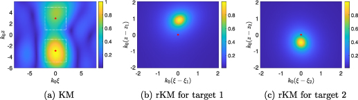
Figure 10. (a) Image produced by KM for an unknown, lossy medium with two targets with noise added to measurements so that  dB. (b) Image produced by rKM with ε = 0.01 in a subregion about the location of target 1. (c) Image produced by rKM with ε = 0.01 in a subregion about the location of target 2.
Download figure:
Standard image High-resolution image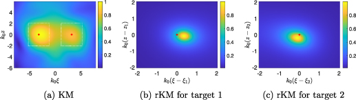
Figure 11. (a) Image produced by KM for an unknown, lossy medium with two targets with noise added to measurements so that  dB. (b) Image produced by rKM with ε = 0.01 in a subregion about the location of target 1. (c) Image produced by rKM with ε = 0.01 in a subregion about the location of target 2.
Download figure:
Standard image High-resolution image
6. Conclusions
We have studied synthetic aperture imaging in a lossy medium. We model absorption in the medium using the loss tangent, which is the imaginary part of the relative dielectric permittivity. Using KM to compute images of targets, we have considered two cases: (i) the loss tangent for the medium is known and (ii) the loss tangent for the medium is unknown.
When the loss tangent of the medium is known and used in KM, we find that images of a point target are range-shifted so that their predicted location is closer to the synthetic aperture than it actually is. The amount by which the target is range-shifted depends on the loss tangent β and the imaging system length L. In contrast, the images produced by KM are relatively unaffected by absorption in cross-range.
In contrast, we have found that when the loss tangent is unknown and not used in KM, the resulting KM images are better. They do not exhibit any range-shifting and their cross-range resolution is the same. In light of these results, we conclude that it is better to not make use of any knowledge of the loss tangent when imaging in a lossy medium.
By applying the recently developed rKM, we are able to achieve tunably high-resolution images of targets. The key is a user-defined parameter ε which can be varied to achieve resolutions that are  in range and
  in cross-range. When there are two or more targets, their predicted locations may shift slightly (a fraction of the central wavelength) in a lossy medium. Because rKM yields such high-resolution images, we find that these shifts become very apparent in rKM images.
Absorption in the medium limits the range over which targets may be imaged. The product  introduces an absorption length scale into the problem. Note that in our results we have normalized all of our images. If
  is too large, then measurements become too small to detect which will affect one's ability to image targets. It is important to recognize this range limitation when imaging in a lossy medium.
This study is limited to the specific case of point sources and targets in a uniformly lossy medium for which the loss tangent is constant. Nonetheless, the results provide valuable insight into more general problems involving extended targets, non-uniform absorption, etc. For this elementary problem, we have shown that making use of knowledge of absorption impairs the localization of targets. Our analysis of this problem suggests that the reason behind this impairment applies to any imaging problem in lossy media—it is in that way that we believe that these results generalize to other related problems. Where knowledge of absorption may become important is in recovering quantitative information on the targets' reflectivity. This is a separate problem and would require different methods.
Acknowledgment
The authors acknowledge support by the Air Force Office of Scientific Research (FA9550-21-1-0196). A D Kim also acknowledges support by the National Science Foundation (DMS-1840265).
Data availability statement
The data that support the findings of this study are available upon reasonable request from the authors.