Comment on 'New variables for 1  +  1 dimensional gravity' (2010 Class. Quantum Grav. 27 025002)

Different sets of canonical variables for 1  +  1-dimensional models of gravity without local physical degrees of freedom have been discussed in [1]. These variables are related to connection formulations as used in classical theories underlying loop quantum gravity. All models of this form are contained in the class of 2-dimensional dilaton models, or equivalently in the class of Poisson Sigma models [2–4]. Since these classes had already been formulated in terms of connection variables [5], there should be a strict relation between the different sets of variables. In this comment we work out the relationship.

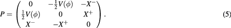
We start with standard formulations of 1  +  1-dimensional actions for a dyad e^a with volume form , a connection 1-form ω and a dilaton field ϕ. For our purpose here, it suffices to consider torsion-free models, such that the condition ${\rm D}e^a=0$, using the covariant derivative given by ω, is implemented by Lagrange multipliers X_a. The dilaton gravity action with potential $V(\phi)$ is then

$$\begin{align} S=-\frac{1}{2G} \int_M \left(\phi{\rm d}\omega+ \frac{1}{2}V(\phi) \epsilon+ X_a{\rm D}e^a\right) \nonumber \end{align} \tag{ 1 }$$

and takes, after integrating by parts, the form

$$\begin{align} S=\frac{1}{2G} \int_M \left(e^a\wedge {\rm d}X_a+ \omega {\rm d}\phi- X_a\epsilon^a_b \omega\wedge e^b- \frac{1}{2}V(\phi)\epsilon\right). \nonumber \end{align} \tag{ 2 }$$

Here, M is a 1  +  1-dimensional manifold with coordinates (t, x).

In Poisson Sigma models, one organizes the variables in new sets $X^i=(X^-, X^+, \phi)$, $A_i=(e_x^+, e_x^-, \omega_x)$, and $\Lambda_i=(e_t^+, e_t^-, \omega_t)$. A canonical analysis leads to Poisson brackets

$$\begin{align} \{X^i(x),A_j(y)\} = 2G\delta^i_j\delta(x-y), \nonumber \end{align} \tag{ 3 }$$

while the $\Lambda_i$ serve as Lagrange multipliers of first-class constraints

$$\begin{align} \label{Ci} \tilde{C}^i = \frac{1}{2G} \left((X^i)^{\prime}+ P^{ij}A_j\right) \nonumber \end{align} \tag{ 4 }$$

with the Poisson tensor [2–4]

$$\begin{align} P=\left(\begin{array}{@{}ccc@{}} 0 & -\frac{1}{2}V(\phi) & -X^- \nonumber \\ \frac{1}{2}V(\phi) & 0 & X^+ \nonumber \\ X^- & -X^+ & 0\end{array}\right). \nonumber \end{align} \tag{ 5 }$$

The variables introduced in [5] are obtained by using the 'absolute values'

$$\begin{align} X:=\sqrt{X^+X^-} \quad{\rm{~and~}}\quad e:=\sqrt{e_x^+e_x^-} \nonumber \end{align} \tag{ 6 }$$

and boost parameters α and β in

$$\begin{align} X^{\pm} = X \exp(\pm\beta) \quad{\rm{~and~}}\quad e_x^{\pm}=e \exp(\pm\alpha). \nonumber \end{align} \tag{ 7 }$$

They are related to the canonical variables

$$\begin{align} \label{Q} Q^e=2X\cosh(\alpha-\beta) \quad{\rm{~and~}}\quad Q^{\alpha}=2eX\sinh(\alpha-\beta) \nonumber \end{align} \tag{ 8 }$$

with

$$\begin{align} \label{PoissonQ} \{Q^e(x),e(y)\}=\{Q^{\alpha}(x),\alpha(y)\}=\{\phi(x),\omega_x(y)\}= 2G\delta(x-y). \nonumber \end{align} \tag{ 9 }$$

The inverse transformation is

$$\begin{align} X^{\pm} = \frac{eQ^e\mp Q^{\alpha}}{2e} \exp(\pm\alpha). \nonumber \end{align} \tag{ 10 }$$

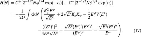
In canonical variables, the constraints are

$$\begin{align} \label{Cpm} \tilde{C}^{\pm} = \frac{1}{2G} \left(\left(\frac{eQ^e\mp Q^{\alpha}}{2e}\right)^{\prime} \pm \frac{eQ^e\mp Q^{\alpha}}{2e} (\omega_x+\alpha^{\prime})\pm \frac{1}{2}V(\phi)e\right)\exp(\pm\alpha) \nonumber \end{align} \tag{ 11 }$$

and

$$\begin{align} \tilde{C}^3 = \frac{1}{2G} (\phi^{\prime}+Q^{\alpha}). \nonumber \end{align} \tag{ 12 }$$

For spherically symmetric gravity, corresponding to a specific dilaton potential $V(\phi)=-2/\sqrt{\phi}$ [4], one can compare the new canonical variables to those used in real connection formulations such as [6], denoted as $(K_{\varphi}, E^{\varphi};K_x, E^x;\eta, P^{\eta})$ and with Poisson brackets

$$\begin{align} \{K_x(x),E^x(y)\}=2G\delta(x-y),\quad \{K_{\varphi}(x),E^{\varphi}(y)\}=G\delta(x-y). \nonumber \end{align} \tag{ 13 }$$

(Note that there is no factor of two in the second equation because the pair $(K_{\varphi}, E^{\varphi})$ represents two angular directions which were independent before symmetry reduction.) They are related to $(Q^e, e;Q^{\alpha}, \alpha;\phi, \omega_x)$ by the canonical transformation

$$\begin{align} Q^e = 2\sqrt{2} (E^x)^{1/4} K_{\varphi},\quad e=\frac{E^{\varphi}}{\sqrt{2}(E^x)^{1/4}} \label{Qee} \nonumber \end{align} \tag{ 14 }$$

$$\begin{align} Q^{\alpha} = P^{\eta},\quad \alpha=-\eta \nonumber \end{align} \tag{ 15 }$$

$$\begin{align} \omega_x = -\left(K_x+\frac{E^{\varphi}}{2E^x}K_{\varphi}-\eta^{\prime}\right),\quad \phi=E^x. \label{omegaphi} \nonumber \end{align} \tag{ 16 }$$

(Unlike the pair $(K_{\varphi}, E^{\varphi})$, the pair (e,Q^e) is defined with a factor of two in the Poisson bracket (9).) These relations have been derived in [5]; see equation (42) in this paper. Also in [5], the spherically symmetric Hamiltonian constraint has been obtained as

$$\begin{align} \label{HDil} H[N] &= C^+[2^{-1/2} N\phi^{1/4}\exp(-\alpha)]- C^-[2^{-1/2} N\phi^{1/4}\exp(\alpha)]\nonumber \\ &= -\frac{1}{2G} \int {\rm d}x N \left(\frac{K_{\varphi}^2E^{\varphi}}{\sqrt{E^x}}+ 2 \sqrt{E^x} K_xK_{\varphi}- \frac{1}{2} E^{\varphi}V(E^x)\right. \nonumber \\ &\qquad\qquad\qquad \left.- \frac{((E^x)^{\prime})^2}{4E^{\varphi}\sqrt{E^x}}+ \frac{\sqrt{E^x}(E^x)^{\prime}(E^{\varphi})^{\prime}}{(E^{\varphi})^2}- \frac{\sqrt{E^x}(E^x)^{\prime\prime}}{E^{\varphi}}\right). \nonumber \end{align} \tag{ 17 }$$

For an arbitrary dilaton potential, this formulation generalizes the connection formulation of spherically symmetric canonical gravity to arbitrary 1  +  1-dimensional dilaton models. Deriving just this kind of result was the aim of [1]. In fact, the definitions of [1] are nothing but the results of [5] with different names chosen for the new variables. The expression for e in (14) is the same as (51) in [1], Q^e in (14) is (57), and $\omega_x$ in (16) is (60).

There is a different formulation in [1] for the specific case of the CGHS model (constant dilaton potential). This model, as presented in [1] has a Hamiltonian constraint with only $K_xK_{\varphi}$ in its kinetic part but no contribution of $K_{\varphi}^2$, unlike what we have in (17). However, this formulation is not new either, even though it does not correspond to a connection formulation as defined in [5]. It rather amounts to using the original canonical variables (8) of dilaton models, along with $\omega_x$, and just renaming them as $\omega_x\equiv K_x$, $Q^e\equiv K_{\varphi}$ and $e\equiv E^{\varphi}$. Except for the new names, these variables, in particular Q^e, have been introduced in [5]; see equation (20) in this paper. Except for using the SU(1,1)-invariant Q^e, they correspond to a first-order formulation of Poisson Sigma models. The constraints (11) in these variables depend on $\omega_x$ in a linear fashion, and so does the Hamiltonian constraint obtained by a linear combination. In these variables, therefore, the Hamiltonian constraint has only one term $Q^e\omega_x=K_xK_{\varphi}$ but not contribution from $K_{\varphi}^2$ (which would amount to $(Q^e){\hspace{0pt}}^2$, but there is no such term in (11)). The quadratic term is introduced in (17) by applying the canonical transformation (14) and (16) via the product $Q^e\omega_x$ in (11).

Even though [1] cites [5], it misses the close relationship between the results.

This work was supported in part by NSF grant PHY-1607414.