
Abstract
Viscoelastic sandwich structures (VSS) are widely used in mechanical equipment; their state assessment is necessary to detect structural states and to keep equipment running with high reliability. This paper proposes a novel manifold–manifold distance-based assessment (M2DBA) method for assessing the looseness state in VSSs. In the M2DBA method, a manifold–manifold distance is viewed as a health index. To design the index, response signals from the structure are firstly acquired by condition monitoring technology and a Hankel matrix is constructed by using the response signals to describe state patterns of the VSS. Thereafter, a subspace analysis method, that is, principal component analysis (PCA), is performed to extract the condition subspace hidden in the Hankel matrix. From the subspace, pattern changes in dynamic structural properties are characterized. Further, a Grassmann manifold (GM) is formed by organizing a set of subspaces. The manifold is mapped to a reproducing kernel Hilbert space (RKHS), where support vector data description (SVDD) is used to model the manifold as a hypersphere. Finally, a health index is defined as the cosine of the angle between the hypersphere centers corresponding to the structural baseline state and the looseness state. The defined health index contains similarity information existing in the two structural states, so structural looseness states can be effectively identified. Moreover, the health index is derived by analysis of the global properties of subspace sets, which is different from traditional subspace analysis methods. The effectiveness of the health index for state assessment is validated by test data collected from a VSS subjected to different degrees of looseness. The results show that the health index is a very effective metric for detecting the occurrence and extension of structural looseness. Comparison results indicate that the defined index outperforms some existing state-of-the-art ones.
Export citation and abstract BibTeX RIS
1. Introduction
Viscoelastic sandwich structures (VSS) comprise a viscoelastic layer confined between two identical elastic and stiff layers [1, 2]. Due to the perfect performance of energy dissipation, VSS are very effective in reducing the vibration and noise of mechanical equipment [3–5]. Hence, the VSS are generally used in fields where low levels of vibration and noise is necessary, such as the aerospace industry and naval forces [6, 7]. During the service of VSS, their health states are changed by temperature, pressure and other influences from the external environment, and hence structural looseness will take place inevitably. Many elements can cause looseness in the VSS, such as the aging of the viscoelastic material and preload relaxation of the connecting bolt. If looseness happens, the structure may be forced to vibrate at the higher amplitude, which will lead to performance degradation of the VSS and even result in failure of the entire mechanical equipment. Where VSS play a role in sealing, looseness would lead to a leakage of the materials stored in the mechanical equipment. Therefore, for the safety and reliability of the VSS, it is important to develop new state assessment technologies in order to identify structural states more accurately [8, 9].
Looseness can be treated as a kind of damage that influences the properties of the VSS, and the methods for damage assessment are generally used to identify the degree of looseness. Damage assessment aims to determine whether the structure is damaged, and if so, the damage can be identified, localized and quantified by damage assessment methods. Damage assessment of the VSS falls within the field of structural health monitoring (SHM). As shown in reference [10], the purpose of SHM is to diagnose the health states of constituent materials, of the different parts and of the full assembly of these parts constituting the structure as a whole, over the entire life span of the structure. SHM is helpful to realize condition-based maintenance and to prevent sudden failure. Considering real-time performance, condition monitoring technologies serve as the foundation of SHM. Lots of condition information, such as acoustic signals, eddy current and vibration signals, has been monitored for structural state assessment [11–13], and useful messages related to damage are extracted from the information to identify structurally damaged states. In practice, vibration response is the most commonly used information for SHM owing to the efficiency and non-destructive property of vibration monitoring. The basic concept of vibration-based structure damage assessment is that damage in the structure will lead to detectable changes in vibration features; a detailed knowledge of vibration-based SHM methods is reviewed in references [11, 14, 15]. Many useful methods have been proposed to implement vibration-based structural damage assessment [3, 16–21]. The methods proposed in these works can be categorized as model-based methods or response-based method. A model-based method assumes that the structure can be modeled as a numerical model, and a finite element model is constructed to investigate the structural dynamic characteristics. For example, Ferreira et al presented a layer-wise finite element model for the analysis of sandwich-laminated plates with a viscoelastic core and laminated anisotropic face layers [3]. Mohammadi et al developed a nonlinear finite element model to investigate the nonlinear vibration properties of sandwich-shell structures [16]. Xiang et al designed a wavelet finite element model to detect damages in the conical shell [17]. The results shown in these papers verify the effectiveness of the model-based method for identifying structural states. While, due to the complexity of structures in practice, simplified models cannot match the actual structural states very well, and this shortcoming limits the accuracy of the solution obtained by the model-based method. Response-based methods deal with damage assessment directly by analysis on the output-only measurement monitored from structures, without the necessity of a dynamical model. For example, Lin et al successfully extracted condition parameters from dynamic response data to assess the instability condition of a bridge structure [18]. Kim et al formulated a damage-sensitive feature from the structural velocity responses for health monitoring of a three-story building structure [19]. Loh et al presented a velocity response analysis method for on-line and almost real-time damage diagnosis of a rigid bridge [20]. Methods of this type assume that patterns in the vibration response are changed when damage happens, and the difference between the signal patterns before and after damage can be extracted and used as a damage index. Hence, response-based damage assessment methods have appealing properties of efficiency.
The idea of response-based damage assessment is often reported by means of subspace identification methods [10, 20–24]. Such methods are nonparametric data-driven methods, and structural damage is detected by pattern analysis on the output-only measurements with no need for identification on modal parameters. In these methods, response signals are used to construct a state matrix, such as a Hankel matrix, to reflect structural dynamic characteristics firstly. A pattern identification algorithm, such as principal component analysis (PCA), is then performed on the state matrix to obtain a subspace. The subspace distance between the baseline subspace and damage subspace is finally taken as a damage index. In recently reported subspace-based damage assessment methods, subspace distance analysis in Euclidean space is a popular choice. For example, Yan et al proposed damage-sensitive features by null subspace analysis of structural vibration acceleration signals, and the norm of the residue matrix is used as a health index [21]. Ren and Lin et al designed new damage features by means of the Euclidean distance and Mahalanobis distance functions [22, 23]. A similar damage detection method was presented by Chao et al [24]. These works show that subspaces are able to capture the essential patterns of response signals, and modeling structural response by subspace analysis has been proven to be an effective way for structural damage detection.
However, there is a drawback in the damage assessment methods based on subspace distance analysis reported in recent works. These methods are single subspace-based processes and ignore the global characteristic across the whole subspace set, which makes the methods only modestly effective when dealing with a mass of subspaces. Recently, a favorable trend is to calculate the distance between two sets of subspaces, by which global characteristics of the subspace set are considered [25]. This method attempts to extract subspace sets from different types of signals and then compare the similarity between the Grassmann manifolds (GM) that are composed of the subspace sets to obtain similarity/distance measures. By doing so, the door for measuring subspace distance in the perspective of global manifold analysis is opened. By global manifold analysis, a novel manifold–manifold distance-based assessment (M2DBA) method is proposed in this paper. In the M2DBA method, subspace sets are analyzed in reproducing kernel Hilbert spaces (RKHS), and a non-Euclidean distance between two subspace sets, that is two GMs, is defined as a health index. In order to implement the M2DBA method, a Hankel matrix is firstly constructed to describe the dynamic characteristics of the signals. Then, the PCA algorithm is used to extract the condition subspace from the Hankel matrix. The subspace from the structural baseline state is called the baseline subspace, and the subspace from a structural looseness state is called the looseness subspace. Next, the subspace set from a structural state constitutes a GM in Euclidean space. Thereafter, a nonlinear mapping function is used to map the manifold from Euclidean space into a RKHS; for a detailed introduction about the RKHS readers can review references [26, 27]. A support vector data description (SVDD) algorithm is performed in the RKHS to model the manifold as a hypersphere that is represented by a radius and a center. A health index is finally defined as the cosine of the angle between the hyperspheres modeled from baseline subspaces and looseness subspaces. That is, five steps—Hankel matrix construction, subspace extraction, Grassmann manifold, SVDD modeling in RHKS and health index definition—are included in the proposed method. The processes of the proposed method are shown in figure 1.
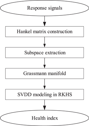
Figure 1. The processes of the proposed M2DBA method.
Download figure:
Standard image High-resolution imageWe continue this paper as follows. Section 2 introduces the fundamental methods used in this paper. Section 3 presents the definition of the health index. The experiment and results are shown in section 4. Comparisons are given in section 5. Conclusions and prospects are summarized in section 6.
2. Methods
In section 1, the proposed M2DBA method is introduced briefly, and the method for the implementation of each step in the method is described in detail in this section.
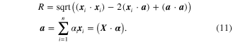
2.1. Hankel matrix construction
As introduced in section 1, construction of a Hankel matrix is a key step in the proposed M2DBA method. For a structure, its discrete-time state space model is constructed by dynamic response as [28]


where  is the d-dimensional state vector at time step
  , and
, and  is the corresponding output vector. The matrix
  is the state matrix and the matrix
  is called the output matrix. The vectors
  and
and  are called state noise and measurement noise respectively. The noise is assumed to be Gaussian white noise with zero mean. For structural subspace identification, the Hankel matrix [10, 21, 29] is defined by the output vector as

where  denotes the covariance-driven Hankel matrix. The parameter p and q are user-defined variables for determining the matrix order, and values of them are equal in this paper. The
  entry
entry  is a covariance matrix, and it is approximately estimated by the output data as

where ![${{M}_{i}}=[{{\tilde{\mathop{z}}\,}_{1}},\cdots ,{{\tilde{\mathop{z}}\,}_{N-i+1}}]$](https://content.cld.iop.org/journals/0964-1726/23/6/065019/revision1/sms493787ieqn11.gif) ,
, ![${{\tilde{\mathop{M}}\,}_{i}}={{[{{\tilde{\mathop{z}}\,}_{i}},\cdots ,{{\tilde{\mathop{z}}\,}_{N}}]}^{T}}$](https://content.cld.iop.org/journals/0964-1726/23/6/065019/revision1/sms493787ieqn12.gif) . N-i + 1 is the number of the output data that are used to calculate
. N-i + 1 is the number of the output data that are used to calculate  and N is the number of all the output data.
2.2. Subspace extraction
To identify the essential data pattern hidden in the Hankel matrix, a pattern recognition method, that is PCA [30], is performed on the Hankel matrix, and a linear subspace spanned by the eigenvector is obtained. The objective function of PCA is an eigenvalue equation described as follows,

where  denotes the covariance matrix.
  is the eigenvalue and
  is the corresponding eigenvector. By solving the eigenvalue equation, we can get
  eigenvectors and eigenvalues. The eigenvectors are orthonormal vectors and they span a linear subspace for the Hankel matrix as

with  denoting the linear subspace.
  is the
  base vector that spans the subspace and
  is dimension of the subspace.
2.3. Grassmann manifold (GM)
A set of linear subspaces can model a GM with each point on the manifold corresponding to a subspace. Local linearity holds everywhere on a globally nonlinear manifold, and global nonlinearity of the GM is represented flexibly by the local linear model. Thus, the Grasssmann manifold G is defined as the set of D-dimensional linear subspaces of  ,
,  and the point on the Grassmann manifold is interpreted as an orthogonal matrix [31]. Formally, the manifold is expressed as

with  denoting the
  component subspace on the manifold, and
  denoting the number of the subspaces. A conceptual illustration for the relationship between subspaces and the GM is shown in figure 2, where
  denotes a subspace in the Euclidean space
  on the left and subspace
  is denoted by a point on the GM on the right.

Figure 2. Conceptual illustration for the relationship between subspaces and GM.
Download figure:
Standard image High-resolution image2.4. Support vector data description (SVDD) modeling of the GM
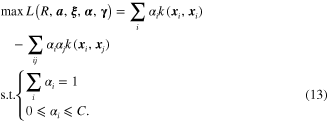
Having defined the GM, the next issue under consideration is how to model the GM reasonably. So, in this subsection, we first introduce the support vector data description (SVDD) in brief and then a GM modeling method by the SVDD is described.
2.4.1. Brief introduction on support vector data description
The SVDD is proposed to deal with the problem of one-class classification [32]. For a data set ![$X=\left[ {{x}_{1}},{{x}_{2}},\cdots ,{{x}_{n}} \right]$](https://content.cld.iop.org/journals/0964-1726/23/6/065019/revision1/sms493787ieqn30.gif) , the SVDD aims to model this data set as a hypersphere
, the SVDD aims to model this data set as a hypersphere  depicted by two parameters, that is the radius
  and the center
  . These two parameters can be obtained by solving the following constrained minimization problem:
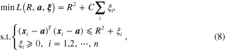
where  is a slack variable to enhance robustness.
  is a penalty factor that gives a trade-off between the volume of the hypersphere and the learning errors. By using the Lagrange multiplier method, the minimization problem is transformed as
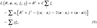
where  and
and  denote the Lagrange multipliers and
  . By calculating the partial derivatives of
  and setting the partial derivatives to be 0, the minimization function in equation (8) can be rewritten as
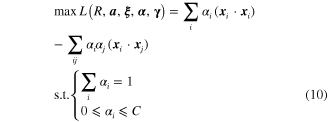
with ![$\alpha ={{\left[ {{\alpha }_{1}},{{\alpha }_{2}},\cdots ,{{\alpha }_{n}} \right]}^{T}}$](https://content.cld.iop.org/journals/0964-1726/23/6/065019/revision1/sms493787ieqn40.gif) . By solving equation (10) the vector
. By solving equation (10) the vector  can be obtained, and then we can get the radius
  and center
  of the hypersphere as
From the two parameters, the data set is modeled to be a hypersphere with explicit expression. Nevertheless, the linear view of SVDD is ineffective when the data set is with a certain degree of nonlinearity. A feasible method to deal with nonlinearity is to map the data set into the RKHS by a nonlinear mapping function φ(·), that is  . In the RHKS, the inner-product is expressed by a kernel function as

where  denotes the kernel function and
  is the nonlinear vector corresponding to vector
  . With the kernel function, the objective function of SVDD in equation (10) is rewritten as
Accordingly, the parameters of the hypersphere modeled by SVDD is extended to be a nonlinear form as
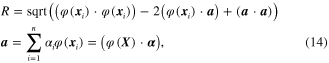
where  is the nonlinear map of the data set, i.e.,
 ![$\varphi \left( X \right)=\left[ \varphi \left( {{x}_{1}} \right),\varphi \left( {{x}_{2}} \right),\cdots ,\varphi \left( {{x}_{n}} \right) \right]$](https://content.cld.iop.org/journals/0964-1726/23/6/065019/revision1/sms493787ieqn49.gif) .
.
2.4.2. GM modeling in reproducing kernel Hilbert spaces (RKHS)
As shown in equation (12), the traditionally used kernel function is the inner-product of a pair of vectors, while the GM is constituted by the subspaces that are organized as matrices. So the challenge for extending SVDD onto the GM is to calculate the kernel function of the subspaces.
Given a GM, that is  , the basic idea of modeling it by SVDD is mainly composed of two steps. The first step is the projection of the manifold from Euclidean space to RKHS by nonlinear mapping φ(·). The next step is to perform SVDD on the GM in the RKHS. After the projection, the GM is written as
  in the RKHS, with
  denoting the nonlinear form of the subspace
  . The objective function of SVDD can be expressed as
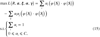
where  denotes the inner-product of two subspaces.
The inner-product of two subspaces can be calculated with the help of the Grassmann kernel that is expressed as

where  is the Grassmann kernel. According to the nature of the kernel function, a function that maps the subspace to be a real-number is an admissible Grassmann kernel if it is real symmetric, positive definite and well-defined for all
  . The real symmetry means that the value of the kernel function is symmetrical, i.e.,
  . The positive definiteness ensures that for all
  , the summation
  is always non-negative. The well-defined property means that value of the kernel function is not changed by different representations of the subspaces, i.e.,
  , with
  and
and  denoting two orthonormal matrices respectively. The reported Grassmann kernel includes the projection kernel and Binet–Cauchy kernel. The Binet–Cauchy kernel [33] is used in this work, and it is of the form of

By submitting the kernel function into equation (15), two parameters of the hypersphere are obtained, and the hypersphere is finally expressed as
where ![$\varphi \left( S \right)=\left[ \varphi \left( {{S}_{1}} \right),\varphi \left( {{S}_{2}} \right),\cdots ,\varphi \left( {{S}_{m}} \right) \right]$](https://content.cld.iop.org/journals/0964-1726/23/6/065019/revision1/sms493787ieqn63.gif) and
and  denotes the hypersphere in the RKHS. A conceptual illustration for the modeling of the GM is shown in figure 3, where
  on the left is the GM in the Euclidean space and the corresponding hypersphere in the RHKS, that is
  , is simply plotted as a circle on the right.
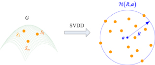
Figure 3. SVDD modeling of GM in the RKHS.
Download figure:
Standard image High-resolution image3. Definition of health index
With the methods described in section 2, vibration signals monitored from the VSS can be modeled to be a hypersphere in the RKHS. In this section, we define the health index by comparing the similarity between hyperspheres from the baseline state and the looseness state, and the physical interpretation of the health index is also revealed.
3.1. The health index (HI)
To design the health index, vibration data are monitored from the structural baseline state and the looseness state respectively. The data are used to form GMs and the GMs are mapped into the RKHS. From the SVDD, hyperspheres of the GMs are modeled. The parameters of the hyperspheres are transformed into a scalar to represent the distance/similarity between the hyperspheres.
For the baseline state, the hypersphere is expressed as  . For the looseness state, the hypresphere is expressed as
  (indicated by superscript ∼). The distance between these two hyperspheres reflects the degree of a looseness state deviating to the baseline state, and it can be used as an index to assess the degree of looseness. Hence, the definition of the health index is equivalent to the measurement of distance between hyperspheres generated from the baseline state and the looseness state. If there is no looseness in the structure, patterns between the data are similar and hence the distance between the hyperspheres should be smaller. Otherwise, structural looseness leads to less similarity between the data patterns, which will generate a larger value in the distance.
The cosine similarity is a commonly used distance/similarity index in the field of pattern analysis, and it is used in this work. For the hyperspheres  and
and  , the cosine of the angle between their centers is defined as a health index (HI), that is,
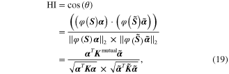
where  is the angle between the centers of the two hyperspheres.
  is the set of subspaces from the baseline state and
  is the set of subspaces from the looseness state in RKHS.
  and
and  are the Lagrange multipliers generated by performing SVDD on the GM corresponding to the baseline state and looseness state respectively.
  is the kernel matrix of
  with the (i, j) entry expressed as

 is the kernel matrix of
  with the (i, j) entry expressed as

 is the mutual kernel matrix of
  and
and  , and its (i, j) element is expressed as

In figure 4, we illustrate the definition of the angle between the two centers intuitively, where  is the hypersphere generated from the structural baseline state with vector
  denoting its center. The hypersphere generated from the structural looseness state is denoted by
  , whose center is expressed as
  . The coordinate origin in the RKHS is expressed as
  and the angle between the two centers is denoted by
  .
.

Figure 4. Conceptual illustration for the definition of the angle between the two centers.
Download figure:
Standard image High-resolution imageIn equation (19), the health index is defined by the inner-product of the subspaces, and the inner-product is formulized easily in the form of a kernel function without an explicit mapping function. The inner-product operation can drive similarity information between two variables, so the defined health index indicates the similarity between the data from the baseline state and looseness state. If the health index is equal to 1, the pattern of the data from a structural state is the same as that from the baseline state, and this state is thought to be without looseness. A larger value of the health index indicates that the two states are more similar, that is to say, the looseness degree is less serious. On the contrary, a health index with a smaller amplitude indicates a structural state with more serious looseness. The smaller the index, the more serious the looseness is.
3.2. Selection of the parameter C
When calculating the health index (HI), a parameter, that is the penalty factor C, should be chosen in the SVDD algorithm. An optimal parameter is viewed as the one that can generate a health index with the best monotonicity. To quantitatively describe monotonicity of the health index, a monotonicity metric is designed as
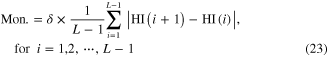
with

where  is the monotonicity metric and
  denotes the number of the structural states. The monotonicity index reflects the slope of the health index, and the factor
  is used to find a parameter that can generate a health index that decreases monotonously. The optimal parameter can be determined by maximizing the following objective function as

with  denoting the optimal parameter.
3.3. Comparison with the reported damage index
To characterize the similarity between the signal subspaces, a health index is defined by considering the global property of the subspace sets. There are some other damage indices, such as the Euclidean distance reported in reference [20], can also be used to reflect the similarity between the signal subspaces. In these indices, the distance between two subspaces is directly calculated without characterizing the global property of the subspace set. This may lead to a performance difference when the defined health index and the reported damage indices are used for damage assessment. Though both the defined health index and the reported indices can reflect the similarity of the subspaces, they reflect subspace similarities in different ways. Hence, it is necessary to analyze the characteristics of the defined health index and the reported indices and to compare their performances for state assessment.
The Euclidean distance is a representative subspace distance metric, and its characteristics are compared with those of the defined health index in the following. Assuming that the subspaces from the baseline state and the looseness state are denoted by ![$S=span\left[ {{s}_{1}},{{s}_{2}},\cdots ,{{s}_{r}} \right]$](https://content.cld.iop.org/journals/0964-1726/23/6/065019/revision1/sms493787ieqn93.gif) and
and ![$\tilde{\mathop{S}}\,=span\left[ {{\tilde{\mathop{s}}\,}_{1}},{{\tilde{\mathop{s}}\,}_{2}},\cdots ,{{\tilde{\mathop{s}}\,}_{r}} \right]$](https://content.cld.iop.org/journals/0964-1726/23/6/065019/revision1/sms493787ieqn94.gif) (indicated by superscript ∼) respectively. The Euclidean distance index (EI) between these two subspaces are calculated as
(indicated by superscript ∼) respectively. The Euclidean distance index (EI) between these two subspaces are calculated as

with

where vec(·) is a column stacking vector with base vectors of the subspaces being connected in order.
It can be seen from equation (26) that the EI is generated from the distance between the base vectors of the subspaces, and the significance of each base vector is considered to be the same for subspace distance measurement. In view of subspace analysis, the significance of the base vector to a subspace is different and it is represented by an eigenvalue that corresponds to the base vector. Not distinguishing the importance of each base vector leads to neglecting the subspace structure in the distance metric. Furthermore, the EI is calculated between two subspaces rather than two subspace sets, and hence the global information of the subspace sets is ignored.
The defined health index is derived from two sets of subspaces with each subspace being treated as a point in the RKHS, and subspace structure and global manifold information are kept in the index. According to the viewpoint of the GM, the GM is generally known as a curved surface, and hence an appropriate metric for measuring distance between a pair of subspaces on it should be the non-Euclidean distance instead of the Euclidean distance. Therefore, a damage assessment method that is based on Euclidean distance may not always work. The proposed health index which identifies structural states in the perspective of global manifold analysis may be more effective.
4. Experiment and results
In this section, an experiment is designed to investigate the vibration characteristics of a VSS subjected to looseness and the vibration signals are used to assess structural health states.
A sketch of the test VSS is illustrated in figure 5(a) and a practical physical structure picture is shown in figure 5(b). It is mainly constituted of metal layers with four layers of silicone embedded in. There is a connecting bolt generating a preload to compress metal layers and silicone layers. To create looseness states, a certain degree of preload is loaded by tightening the nut to create a baseline state. The preload is then decreased gradually by loosening the nut to create five looseness states with the assumption that a smaller preload will generate a more severe looseness state. As shown in figure 6, five looseness states are denoted by LS1–LS5, respectively, and the baseline state is denoted by BS. In looseness state 1 (LS1), the preload is decreased by 1000 N from the baseline state. By that analogy, in states LS2-LS5, the preload is decreased by 2000 N, 3000 N, 4000 N and 5000 N from the baseline state respectively. It can be seen that looseness degrees in the five states are gradually deepening.
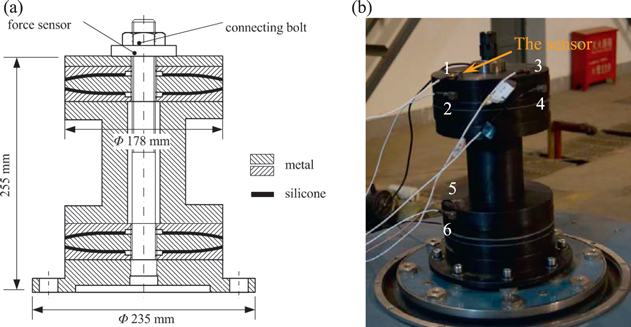
Figure 5. The sketch and the photo of the viscoelastic sandwich structure. (a) The sketch. (b) Practical physical structure picture, 1–6: location of the sensors.
Download figure:
Standard image High-resolution image
Figure 6. Definition of the six structure states.
Download figure:
Standard image High-resolution imageThe structure is randomly excited by a vibration exciter table in the vertical direction as shown in figure 7. The excitation signal is in the frequency range of 0–2000 Hz, and the power spectrum density (PSD) of the signal is shown in figure 8. Six acceleration sensors are mounted on the surface of the structure, with three of them measuring the vibration signals from the axial direction and the other three from the radial direction. Under the excitation, vibration response signals of the structure in all health states are monitored by the six sensors and then stored by a data acquisition system. The sampling frequency is set to be 10 240 Hz and the sampling time for each state is 2 min.

Figure 7. The external view of the test bench.
Download figure:
Standard image High-resolution image
Figure 8. Power spectrum density (PSD) of the excitation signal.
Download figure:
Standard image High-resolution imageAfter data acquisition, acceleration response signals from sensor 2 are plotted in figure 9. These acquired signals are entered in the M2DBA method to investigate structural health states. When performing the proposed method, the response signals from each structural state are divided into 60 segments with each segment consisting of 20 480 × 6 data points. Data points from each segment are utilized to establish a Hankel matrix. Numbers of row block  and column block
  in it are set equally to 10. Then, the Hankel matrix is decomposed by the PCA algorithm, and the obtained eigenvectors are used to span the condition subspace. After that, a GM is constructed by using a set of subspaces and the manifold is mapped into the RKHS where it is modeled by the SVDD algorithm to obtain a hypersphere. In the SVDD algorithm, the optimal parameter C is searched for from the potential parameters in the range of
 ![$\left[ {{2}^{-15}},{{2}^{15}} \right]$](https://content.cld.iop.org/journals/0964-1726/23/6/065019/revision1/sms493787ieqn97.gif) with the search step length equaling 2. The health index generated from some of the potential parameters is shown in figure 10. To search the optimal parameter, the monotonicity metric of the health index generated from all the parameters is calculated and it is shown in figure 11(a). It can be seen that the monotonicity metric of the health index is less than 0 when parameter C is equal to
with the search step length equaling 2. The health index generated from some of the potential parameters is shown in figure 10. To search the optimal parameter, the monotonicity metric of the health index generated from all the parameters is calculated and it is shown in figure 11(a). It can be seen that the monotonicity metric of the health index is less than 0 when parameter C is equal to  . This indicates that the corresponding health index is not decreasing monotonously, which can be seen in figure 10. The health index generated from the other potential parameters is decreasing monotonously with the increase of the looseness degree. The monotonicity metric reaches maximum when parameter C is equal to
  , as shown in figure figure 11(b), and the optimal parameter is chosen as
  .
.
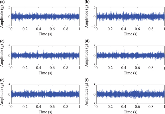
Figure 9. Response signals under all the structural states monitored by sensor 2. (a) Baseline state. (b)–(f) Looseness states 1–5.
Download figure:
Standard image High-resolution image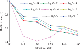
Figure 10. The health index generated from some of the potential parameters.
Download figure:
Standard image High-resolution image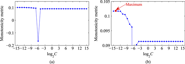
Figure 11. Monotonicity metric of the health index generated from all the potential parameters.
Download figure:
Standard image High-resolution imageBy using the searched optimal parameter, the health index for all the structural states are finally calculated by similarity analysis between the hyperspheres. State assessment for the baseline state is carried out by calculating the similarity between the subspace set from the baseline state and itself. The health index for a looseness state is obtained by calculating the similarity between the baseline subspace and the looseness subspace. The obtained health index is listed in table 1 and shown in figure 12. In figure 12, we plot the structural states on the x-axis and the health index on the y-axis. It can be seen that the health index for the baseline state is equal to 1 and it is less than 1 for all the looseness states. The looseness state 1 (LS1) leads to an obvious decrease in the health index, which demonstrates the health index is sensitive to the occurrence of the looseness. Moreover, a more serious looseness state corresponds to the health index with a smaller value. The decreasing trend in the health index indicates an increasing degree of looseness.
Table 1. The calculated health index for all the structural states.
| Structural state | ||||||
|---|---|---|---|---|---|---|
| BS | LS1 | LS2 | LS3 | LS4 | LS5 | |
| Health index (HI) | 1 | 0.71 | 0.69 | 0.57 | 0.54 | 0.49 |
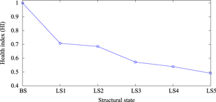
Figure 12. Health index for all the structural states.
Download figure:
Standard image High-resolution image5. Comparisons
5.1. Comparison with statistical indices in the time domain and frequency domain
Pattern analysis in the time domain and frequency domain is a commonly used approach to identify the health of mechanical structures. Some indices, such as kurtosis, can be extracted to describe the properties of vibration signals. In our previous work [34], a damage assessment method was proposed based on these indices, which are also successfully used to describe the dynamic characteristics of vibration signals monitored from the mechanical components, such as bearing and gear [35–38]. To verify the effectiveness of the proposed health index, some classical statistical indices are investigated and their performance for distinguishing degrees of looseness is compared with that of the proposed health index (HI).
Average values of the indices in the time and frequency domains from all the sensor signals are calculated and normalized. Change trends of the normalized indices in the time domain and frequency domain along with the looseness are shown in figure 13. These three indices capture the pattern properties of vibration signals from different perspectives. The index  is a metric that measures Gaussian properties within the signals in the time domain. The index
  describes the convergence of the spectrum power in the frequency domain. The index
  shows the main frequency band of the signals. Formulas for computing these indices are listed in reference [34]. It can be seen on one hand that the sensibilities of these three statistical indices are different for state identification. On the other hand, the trend in each index changes dissimilarly, which shows pattern variety hidden in the vibration signals. Furthermore, there is no obvious change trend in index
  and
and  . The value of index
  for looseness state 4 (LS4) is bigger than that for looseness state 3 (LS3), and hence this index fails to distinguish these two states. In comparison, the monotonous decreasing trend in the proposed health index (HI) is more effective for distinguishing the looseness degree. Hence, the proposed method in this work dealing with state assessment by analyzing pattern variations in the signal subspace is more available and useful.
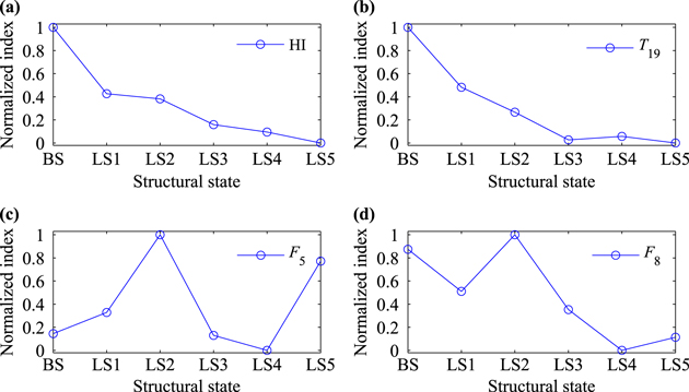
Figure 13. Comparison of the health index with the indices in the time domain and frequency domain.
Download figure:
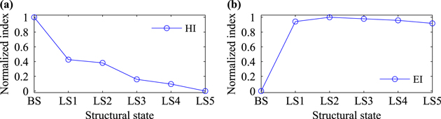
Standard image High-resolution image5.2. Comparison with the reported damage index
As stated in section 3.3, the characteristic of the defined HI is different from that of the reported EI, which would lead to performance differences when they are used for state assessment. For the purpose of comparison, this EI is also calculated from the test data. The variational ranges of the HI and EI are not the same, so the normalization is performed to transform them into the same scale.
The obtained normalized indices are shown in figure 14. It can be seen that, the EI increases distinctly when looseness state (LS1) occurs, which indicates that the EI is sensitive to distinguishing the baseline state from the looseness states. However, the EI cannot distinguish the five looseness states very well and there is no obvious increasing trend in the value of EI. Compared with the EI, the defined HI is more effective to reveal the change of the structural states.
Figure 14. Comparison of HI with EI.
Download figure:
Standard image High-resolution image
6. Conclusions and prospects
With the aim to assess looseness states in viscoelastic sandwich structures, a novel manifold–manifold distance-based (M2DBA) method is proposed by analysis of structural response signals. In the method, the distance between two GMs is designed as a health index. Application results of the method show that the proposed health index indicates initial looseness with a significant reduction in its amplitude, and the tendency in the index monotonously decreases with the increase of the looseness degree. As a result, the proposed method is very effective to assess the degree of looseness of the viscoelastic sandwich structure.
The performance of the defined health index is compared with that of the statistical indices in the time domain and frequency domain. Due to pattern variety in the response signals, the single index that describes signal characteristics from a certain aspect cannot detect looseness reasonably. All the pattern changes of the response signals are described in the signal subspace, and hence the proposed health index is more effective than the indices in the time domain and frequency domain to detect structural health states. Moreover, the defined health index is compared with the recently reported index. During the construction of the index, the subspace structure of the signals is destroyed, so it cannot detect looseness correctly. On the contrary, the proposed health index pays attention to the global properties of the subspaces by treating the subspace set as a Grassmann manifold. Global and structural information of the subspaces is contained in the defined health index, so it is more useful than the reported index to identify structural health states. The comparison indicates that the proposed method is a very effective method for structural state assessment.
In order to assess looseness in the VSS, looseness states are created by reducing the preload of the connecting bolt. While the proposed M2DBA method is a generally used method for state assessment, and with further application the method can be extended to assess structural looseness states due to other causes, such as aging and embrittlement in viscoelastic material. In addition, the structure is excited in the vertical direction in this study. In practice, structure excitation may also be in other directions. The type of the excitation may affect damage assessment results, and hence an investigation on the influence of excitation direction to the results is a potential future research point.
Acknowledgements
The authors would like to express appreciation to the reviewers and editors for their valuable comments to improve the paper. The authors are very grateful to the joint support of the NSAF of China (grant no.11176024), National Natural Science Foundation of China (no. 51275382), Research Fund for the Doctoral Program of Higher Education of China (no. 20110201130001), National Basic Research Program of China (no. 2011CB706805), Postdoctoral Science Foundation of China (no. 2013M532032) and Doctoral Foundation of Education Ministry of China (no. 20130201120040).