
Abstract
Spin-stabilization of spacecraft immensely supports the in-flight calibration of on-board flux-gate magnetometers (FGMs). From 12 calibration parameters in total, 8 can be easily obtained by spectral analysis. From the remaining 4, the spin axis offset is known to be particularly variable. It is usually determined by analysis of Alfvénic fluctuations that are embedded in the solar wind. In the absence of solar wind observations, the spin axis offset may be obtained by comparison of FGM and electron drift instrument (EDI) measurements. The aim of our study is to develop methods that are readily usable for routine FGM spin axis offset calibration with EDI. This paper represents a major step forward in this direction. We improve an existing method to determine FGM spin axis offsets from EDI time-of-flight measurements by providing it with a comprehensive error analysis. In addition, we introduce a new, complementary method that uses EDI beam direction data instead of time-of-flight data. Using Cluster data, we show that both methods yield similarly accurate results, which are comparable yet more stable than those from a commonly used solar wind-based method.
Export citation and abstract BibTeX RIS

Content from this work may be used under the terms of the Creative Commons Attribution 3.0 licence. Any further distribution of this work must maintain attribution to the author(s) and the title of the work, journal citation and DOI.
1. Introduction
The in-situ characterization of the magnetic field in space has been a major objective of numerous spacecraft missions. For that purpose, flux-gate magnetometers (FGMs) are commonly used due to their superior accuracy, stability, and robustness, paired with their relatively low mass and power demand, e.g. [1, 4].
The primary output of FGMs are raw vectorial magnetic field measurements  in sensor coordinates. These need to be transformed into physically meaningful units and coordinate systems, e.g. with the following equation:

Here,  represents the calibrated magnetic field measurements,
  is a 3 × 3 matrix dependent on six angles that transforms from sensor coordinates to an orthogonal, spacecraft-fixed coordinate system,
  is a diagonal matrix consisting of three gain parameters, and
  is a 3D offset vector. Altogether,
  ,
,  , and
, and  are dependent on 12 parameters (6 angles, 3 gains, and 3 offsets) that have to be determined by ground-based (pre-launch) or in-flight (post-launch) calibration procedures, e.g. [3, 9, 11, 21].
The vector  may exhibit larger variations due to spacecraft contributions: the vector represents the FGM measurement in zero ambient field, i.e. to a major extend, the stray fields of the spacecraft on which the FGM is mounted. These fields result from remanently magnetized parts and/or electric currents, e.g. [14]. Changes thereof that directly affect
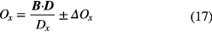
  can only be accounted for by in-flight calibration.
Fortunately, the in-flight calibration procedures are relatively easy for spacecraft that are spin-stabilized. In that case, 8 of the 12 calibration parameters influence the measurements' spectral power at spacecraft spin frequency and/or harmonics in any inertial (de-spun) coordinate system, e.g. [2], which facilitates their in-flight determination. Out of these eight parameters, two are the spin plane components of  , which we denote as Oy and Oz. However, determining the spin axis offset Ox (spin axis in x direction) is much more difficult.
Usually, Ox is obtained by analyzing solar wind (SW) FGM measurements that contain Aflvénic disturbances, i.e. field rotations without changes in field strength, e.g. [10, 13, 18]. Alternatively, simultaneous observations from an electron drift instrument (EDI) may be used. EDI consists of two gun-detector units (GDUs) mounted on opposite sides of a spacecraft. Each GDU can emit modulated electron beams. The electrons perform one (or more) gyrations in the ambient magnetic field and are registered by the other GDU. The electron time-of-flight (TOF) T is in principle inversely proportional to the field strength:
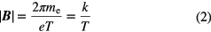
Here, me is the relativistic electron mass, e is the elementary charge, and k = 2π me/e. Differences in T as measured by both GDUs indicate the presence of an electric field or magnetic field gradient [17, 19]. Since measurements of  by an EDI are independent from spacecraft stray fields, they can be used to determine Ox: A correction to this offset is given by the difference between FGM and EDI measured
  , if the field points in spin axis direction. In this paper, we denote such a method of determining or adjusting Ox via EDI TOF measurements as time-of-flight method (TOF method).
An early description of the TOF method can be found in [8]. Later [12] explored the possibility of determining some of the parameters of matrix  by a comparison of FGM and EDI measurements. Just recently [15] showed that the EDI TOF data are also subject to offsets, which systematically alter the Ox results by the TOF method. These studies proved the feasibility of the TOF method, but fell short of presenting a mature method for FGM spin axis offset determination using EDI measurements, which takes into account TOF offsets and other inaccuracies in FGM and EDI observations.
The importance of such a method and timeliness of its development is rooted in its relevance for NASA's upcoming Magnetospheric Multi-Scale (MMS) mission. The mission consists of four spacecraft (featuring FGM and EDI instruments) that will explore the Earth's magnetosphere. The primary objective of the mission is to investigate the physics of magnetic reconnection. During the first years of operation, the MMS spacecraft will rarely encounter the pristine SW, if at all, as their apogee distances from Earth will be too low. Hence, MMS will rely on the availability of a working, mature, EDI-based method for spin axis offset calibration.
The purpose of this paper is to make a major step forward in the development of such a method. First, we provide the TOF method with a comprehensive error analysis that facilitates the determination of spin axis offsets with higher accuracy. Secondly, we introduce another, complementary method which makes use of EDI beam direction (BD) data instead of TOF data. Consequently, we denote this method as beam direction method (BD method). Finally, we compare the spin axis offset results of the TOF method, of the BD method, and of a typically used solar wind (SW) based method [13], which is henceforth denoted as SW method. The data set we base this comparison on consists of one year (2008) of Cluster 3 FGM and EDI measurements.
2. Methods
Apart from the spin axis offset Ox, we assume the FGM measurements to be well-calibrated. Furthermore, we assume that for every EDI measurement there is a simultaneous FGM observation  available. We would like to point out that the methods described in this section provide spin axis offsets Ox after equation (1) if the FGM observations
  are initially computed from
  using Ox = 0. Otherwise, Ox denotes a correction to the already applied spin axis offset rather than the entire offset itself.
2.1. TOF method
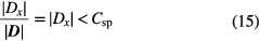
Step 1: In order to avoid systematic errors in Ox, the EDI GDU and operation mode dependent TOF offsets have to be corrected first, as shown by Nakamura et al [15]. For this purpose, measurements need to be selected for which  is unaffected by Ox (magnetic field close to the spin plane, i.e. y-z-plane):
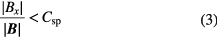
Here Csp is a threshold value; Bx and  are FGM-measured quantities. From the selected FGM and simultaneous EDI data, differences δT between FGM-determined magnetic field strengths, converted to TOFs, and EDI measured TOFs are computed:
Therewith, we obtain one TOF offset OT per GDU and operation mode:


Note that OT is specific to each GDU and operation mode. Hence, for the computation of each offset OT only samples δT corresponding to the particular GDU and obtained when the instrument was in the respective mode may be used.
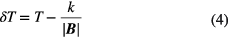
Step 2: All TOF values T (belonging to a particular GDU and mode, not restricted by Csp) are subsequently corrected with the corresponding TOF offsets OT:


Therewith, estimates of the FGM spin axis offset (correction) Ox can be computed:
The uncertainty ΔOx of each Ox estimate does not only stem from ΔTc, i.e. from the TOF offset computations, but also from the inherent FGM measurement and calibration uncertainty of  . Inaccuracies in
  and
and  will result in errors of
  that scale with the strength of the magnetic field. Furthermore, there is a FGM noise floor which defines a minimum uncertainty of
  . Taking both uncertainties into account, we assume each component of
  to be associated with an error of the following form:

where Δg is a factor of unit 1 and ΔBn is the noise level in nT. From equations (9) and (10) we derive the error of Ox (error propagation):
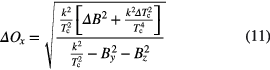
As can be easily seen, ΔOx increases with the factor:
Consequently, it is advantageous for spin axis offset determinations with the TOF method if the field is low in strength and directed along the spin axis.
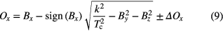
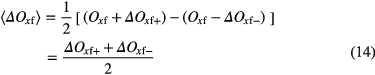
Step 3: The samples of Ox (and corresponding ΔOx) are the basis for the computation of a final offset (correction) value Oxf for a specific time interval of length tint. Therefore, we select those Ox within the time interval, for which ΔOx ⩽ CO holds (CO is a threshold value), and compute:

with upper/lower error bounds given by the 16th and 84th percentiles Oxf − ΔOxf− and Oxf + ΔOxf+ of the distribution of selected/contributing Ox, if their number exceeds another threshold number C#. The percentiles yield a 2σ range around the mean, if the estimates Ox are normally distributed, but also account for skewness of the distribution. The average error of Oxf is given by:
Clearly, the choice of tint, CO, and C# will influence the result Oxf. Larger intervals increase the statistical basis at the expense of a larger spread of the Ox estimates due to offset drift. Lowering CO and increasing C# will also increase the quality of Oxf in general, but less intervals of length tint may fulfill the criteria and yield such an offset value.
It should be noted that realistic uncertainties ΔOx facilitate the selection of the most accurate estimates Ox for the computation of a final offset (correction) Oxf. Hence, error analysis is not only necessary to assess the uncertainty of any result, but is also crucial, in this case, for maximizing the result's accuracy.
2.2. BD method
Only those electron beams, that are emitted by an EDI GDU perpendicular to the ambient magnetic field, are able to return to the spacecraft. Hence, EDI beam directions (BD), which we denote with  , should be perpendicular to
  . Deviations in angles α (depicted in orange in figure 1) between FGM measured
  and EDI measured
  from 90° may be attributed to inaccuracies in spin axis offset Ox.

Figure 1. Sketch illustrating the angles between distinguished directions. Note that  and
and  have non-vanishing y-components (out of the figure plane), in general.
Download figure:
Standard image High-resolution imageStep 1: BDs are not subject to TOF offsets. However, for any BD method to yield accurate spin axis offsets, the coordinate systems of the BDs and of the calibrated FGM data have to coincide. Any adjustment of the coordinate systems should be based on FGM and EDI measurements for which the angles α are least affected by the spin axis offset  close to the spin plane). Our selection criterion is:
where  . Therewith, GDU specific coordinate transformations for the EDI BDs are found by minimization of the mean of (α −90°)2. The standard deviation

can be regarded as angular uncertainty of the BD vectors  . The target coordinate systems should ideally coincide with the coordinate system of the calibrated FGM measurements. All the EDI BDs
  (not restricted by Csp) are transformed into these systems.
Step 2: Ideally,  , as stated above. Deviations can be attributed to the FGM spin axis offset as follows:
Here, the uncertainty ΔOx results from the uncertainties of the components of  (after equation (10)) and of the components of
  :
:

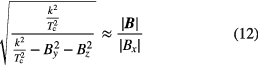
Note that Δβ and, hence, ΔD are GDU specific. Therewith, we obtain the error in Ox in a similar manner to equation (11):
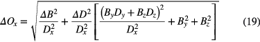
Here ΔB and ΔD are computed in accordance to equations (10) and (18), and  . As can be seen, ΔOx increases with decreasing
  and also with increasing
  , as:
, as:
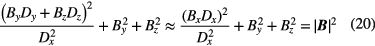
The reason for this behavior stems from the sensitivity of α to changes in Ox being given by the quotient of the two quantities  and
and  :
:
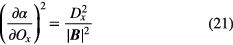
Consequently, it is advantageous for spin axis offset determinations with the BD method if the field is low in strength and pointing in perpendicular direction to the spin axis.
Step 3: Following the description of step 3 of the TOF method, a final spin axis offset (correction) value Oxf for a time interval of length tint can be computed from Ox estimates pertaining to that interval, for which ΔOx < CO holds, via:

if their number exceeds a minimum threshold of C#. Upper/lower error bounds Oxf − ΔOxf− and Oxf + ΔOxf+ may again be given by the 16th and 84th percentiles of the distribution of selected/contributing Ox, with equation (14) defining the average error 〈ΔOxf〉 of the final spin axis offsets (or offset corrections) Oxf.
2.3. SW method
Magnetic field fluctuations embedded in the solar wind (SW) are primarily Alfvénic in nature, i.e. the field changes rather in direction than in magnitude. Hence, the magnitude of the magnetic field tends to be more constant over time than any of its three components [16]. The spin axis offset of a FGM can be determined in the solar wind by making use of this property, as incorrect offsets lead to an artificial increase in fluctuation levels of the field magnitude [1, 5, 6, 10, 20]. The technique used herein introduced and described in [13] is an improved and automated version of the Davis–Smith method [6]. Henceforth, it is referred to as SW method. This method relies on a few hours of FGM solar wind data as input, and yields final spin axis offset (correction) values Oxf (O3 in [13]) as well as upper and lower error bounds Oxf − ΔOxf− and Oxf + ΔOxf+ (O3min and O3max in [13]), just as the TOF and BD methods.
3. Application
We apply the TOF, the BD, and the SW methods to one year (2008) of Cluster 3 EDI and FGM measurements. The FGM measurements were calibrated using the daily calibration files [7]. Roughly 25 million EDI data samples (i.e. combinations of  , T, as well as corresponding simultaneous FGM measurements
  are available for that year.
It should be noted that the daily calibration files include a non-vanishing spin axis offset, which remains constant throughout the year 2008. Consequently, all values Ox that are determined by the TOF, the BD, and the SW methods are corrections to that daily calibration file spin axis offset.
3.1. TOF method
Step 1 consists of the determination of GDU and EDI mode dependent TOF offsets. For this task, we selected EDI and FGM measurements in accordance to equation (3) with Csp = 0.1. Two oppositely directed GDUs are placed on each Cluster spacecraft. The mode of each of these units is characterized by three parameters: n, m, and the code flag f. These parameters control the pseudo noise sequence of electrons emitted by each GDU. A sequence may consist of either 15 (short code, f = 0) or 127 chips (long code, f = 1). The chip length is given by the product of n and m, which are dividers of the internal EDI clock. Although EDI can in principle emit electrons at different energies, only one energy level was used (1 keV). The corresponding relativistic conversion factor between TOF and magnetic field values is k = 35 793.785 µs nT [17].
During 2008, both Cluster 3 GDUs were operated in modes characterized by n ∈ [1, 2, 4, 8, 16, 32] and m = 8 or 16. As EDI is a system of 2 GDUs, each being able to emit modulated electron beams with 2 different code lengths, with chip lengths given by 6 × 2 combinations of m and n, in total 2 × 2 × 6 × 2 = 48 different TOF offsets OT need to be considered. However, for some parameter combinations, there are very few measurements left (less than 100), having taken into account equation (3). In these cases, we abstain from computing OT and disregard measurements of the respective modes for the following TOF method computations. For all other parameter combinations, TOF offsets OT and uncertainties ΔOT are listed in table 1.
Table 1. TOF offsets and uncertainties OT ± ΔOT (in μs) dependent on GDU (1 or 2) and EDI mode (code length f and clock dividers n and m).
| n | m | OT ± ΔOT (μs) | |||
|---|---|---|---|---|---|
| GDU 1 | GDU 2 | ||||
| f = 0 | f = 1 | f = 0 | f = 1 | ||
| 1 | 8 | — | — | — | — |
| 2 | 8 | — | — | — | — |
| 4 | 8 | −0.412 ± 1.330 | — | −0.955 ± 1.110 | −0.459 ± 1.273 |
| 8 | 8 | −0.885 ± 1.747 | — | −1.415 ± 1.752 | — |
| 16 | 8 | −0.142 ± 3.649 | — | −0.898 ± 3.629 | — |
| 32 | 8 | −1.004 ± 3.228 | — | −1.252 ± 8.972 | — |
| 1 | 16 | 0.006 ± 0.103 | −0.018 ± 0.206 | −0.259 ± 0.188 | −0.245 ± 0.191 |
| 2 | 16 | — | −0.059 ± 0.406 | −1.117 ± 1.067 | −0.289 ± 0.439 |
| 4 | 16 | — | −0.435 ± 1.149 | — | −0.522 ± 1.118 |
| 8 | 16 | −0.477 ± 0.693 | −0.264 ± 2.699 | −0.684 ± 0.903 | −0.535 ± 2.673 |
| 16 | 16 | — | 0.107 ± 4.503 | — | −0.246 ± 6.329 |
| 32 | 16 | — | — | — | 3.327 ± 19.23 |
For step 2, assumptions with respect to Δg and ΔBn are required. Orthogonalization angles and gains (matrices  and
and  are assumed to be accurate to the order Δg = 10−4. The noise level of the Cluster FGMs is on the order of ΔBn = 10 pT. Therewith, we obtain uncertainties ΔOx via equation (11). They are color coded in figure 2 and depicted as a function of
  and the angle ξB (blue in figure 1) between
  and the spin axis x. As expected, the uncertainties ΔOx decrease with
  and ξB. Hence, low ΔOx are found in the lower left corner of that figure.

Figure 2. ΔOx, resulting from the application of the TOF method to Cluster 3 EDI and FGM measurements from 2008, as a function of  and the angle ξB between
  and the spin axis x.
Download figure:
Standard image High-resolution imageThe value of Δg = 10−4 reflects the order of magnitude of long term variations of those calibration parameters, influencing  and
and  , that can be accurately determined in flight (e.g. the ratio of the spin plane component gains). However, some calibration parameters that influence
  , as measured by the FGM, namely the absolute spin axis and spin plane gains, cannot be easily and/or accurately determined in flight. It has to be assumed, without possibility of verification, that their long term variations are of the same order of magnitude. Consequently, FGM measurements are not guaranteed to exhibit relative accuracies on the order of or better than Δg = 10−4. Nevertheless, for the purpose of spin axis offset determination, we necessarily have to assume that the only undetermined calibration parameter is, indeed, Ox.
In step 3, we compute Oxf for sliding windows of tint = 15 min shifted by 5 min. The quality thresholds were set to CO = 0.2 nT and C# = 100, respectively. Therewith, we obtain 3523 final offset correction values Oxf distributed over 68 different orbits. The distribution of Oxf values is depicted by a red line in figure 3(c).

Figure 3. (a) Numbers of EDI samples (i.e. BD and TOF measurements) per orbit. (b) Lines connect minimum and maximum  values corresponding to EDI measurements. (c) Numbers of values Oxf per orbit as obtained by the TOF method (red lines) and by the BD method (green bars). Orbits for which a spin axis offset could be determined by the SW method are marked by black arrows.
Download figure:
Standard image High-resolution imageThe figure illustrates how a number of EDI measurements per orbit (panel (a)) taken at certain  conditions (panel (b)) is converted into a number of final offset correction values Oxf (red line, panel (c)). Interestingly, Oxf values were computed roughly for every second orbit. This can be easily explained: For Oxf computations, we selected Ox estimates that fulfill ΔOx ⩽ CO = 0.2 nT. As shown in figure 2, these estimates are obtained in significant numbers for magnetic field strengths below 60 nT. EDI measurements in this field range were taken roughly during every second orbit (see figure 3(b)). For those orbits, Oxf values are computed.
3.2. BD method
Each GDU can emit electrons in a solid angle range larger than 2π around a central axis. On Cluster, this axis is perpendicular to the spin axis. For convenience, we assume it to point in z-direction. For angles ζD between  and z (shown in green in figure 1) approaching or even surpassing 90°, the beam width is known to increase significantly. This effect would deteriorate the results of the BD method. Therefore, we exclude EDI measurements with ζD > CD = 80°.
For the coordinate system adjustment (step 1 of the BD method) we select EDI (and corresponding FGM) measurements for which Dx < Csp = 0.1 holds (equation (15)). Minimal deviations on the order of 0.6° are found between the coordinate system transformations that are obtained from EDI/FGM data comparison and the nominal transformations that are given by the Cluster spacecraft building plans. The angular uncertainties of the former transformations are Δβ = 0.25° for GDU 1 and Δβ = 0.28° for GDU 2.
Again, we assume Δg = 10−4 and ΔBn = 10 pT. The resulting uncertainties ΔOx are shown in figure 4, this time as a function of  and the angle ξD between
  and the spin axis x (depicted in red in figure 1). Figure 4 is somewhat similar to figure 2 as lower uncertainties ΔOx are also found in the lower left corner, corresponding to lower field values
  and lower angles ξD (i.e.
  close to the spin axis). However, for equal field values
  minimal uncertainties ΔOx are larger for the BD method than for the TOF method.
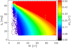
Figure 4. ΔOx, resulting from the application of the BD method to Cluster 3 EDI and FGM measurements from 2008, as a function of  and the angle ξD between
  and the spin axis x. Note that EDI measurements with ξD < 10° are excluded, as they also fulfill ζD > CD = 80° (see figure 1).
Download figure:
Standard image High-resolution imageThe final offset correction values Oxf are computed for tint = 15 min sliding windows shifted by 5 min, CO = 0.2 nT, and C# = 100. Therewith we obtain 2792 values Oxf distributed over 46 orbits. The numbers of these values per orbit are depicted in figure 3(c) by green bars.
3.3. SW method
In 2008, the apogee distances of Cluster 3 to the Earth's center were larger than 20 Earth radii. Hence, dayside apogee positions were beyond the bow shock, in the pristine solar wind (SW). Due to the Earth's rotation around the Sun, the apogee positions rotated once around Earth over the course of the year. When they were at the night side, Cluster 3 stayed inside the magnetosphere and the SW was not observed. Consequently, SW measurements were performed by Cluster 3 not during the entire year, but are available just for the first 6 months and for December of 2008.
We applied the SW method to the solar wind (spin averaged) FGM measurements of each orbit, if available. Specifically, we used the parameters and criteria given in the 'THEMIS' column of table 1 of [13]. As a result, we obtained 53 spin axis offset corrections Oxf pertaining to 53 different orbits (49 for DOYs 2–150, and 4 for DOYs 357–364). The corresponding solar wind data intervals ranged between 32 and 57 h in length. Orbits for which a final spin axis offset correction Oxf could be computed by the SW method are marked by black arrows in figure 3(c).
4. Results and discussion
The Oxf results of the three methods are shown in figure 5(a) (red dots: TOF method, green dots: BD method, black crosses: SW method). In total, 6368 Oxf values contribute to that figure: 3523 from the TOF method, 2792 from the BD method, and only 53 from SW method. The results show consistently that the spin axis offset (as part of the FGM calibration files for that year) is, in general, off by about −0.2 nT. This systematic deviation is expected as the spin axis offset value in the calibration files for 2008 was determined in 2003. Since then, the offset has been checked periodically, but has been kept constant, as its changes were found to lie within its margins of error (Fornaçon, personal communication). Consequently, deviations of Oxf from 0 reflect the long term offset drift in spin axis direction from 2003 to 2008.
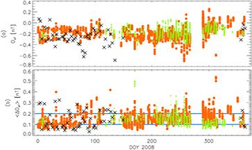
Figure 5. (a) Final spin axis offset corrections Oxf obtained by the TOF method (red dots), the BD method (green dots), and the SW method (black crosses). (b) Corresponding average errors 〈ΔOxf〉 after equation (14). The blue lines mark 〈ΔOxf〉 = 0.1 nT and 0.2 nT levels (see text for details).
Download figure:
Standard image High-resolution imageMedian values of Oxf are −0.20 nT (TOF method), −0.15 nT (BD method), and −0.26 nT (SW method). The corresponding standard deviations are 0.11 nT, 0.08 nT and 0.15 nT, respectively. Taking into account these standard deviations, in particular of the SW method results, we have to regard the median spin axis offset corrections resulting from the three methods as quantitatively similar.
The average errors 〈ΔOxf〉 (after equation (14)) of all Oxf values are depicted in figure 5(b). The minima and maxima of this quantity are 0.05 and 0.53 nT (TOF method), 0.06 and 0.59 nT (BD method), as well as 0.04 and 0.32 nT (SW method). The medians of 〈ΔOxf〉, which are more representative of the typical uncertainties, are 0.14, 0.12 and 0.12 nT for the TOF, BD, and SW method offsets, respectively. Hence, they are practically equal. If the margins of error of the results from the different methods are associated with similar statistical confidence levels, then the accuracies of the results obtained with the three methods will be practically equal, on average, as well.
The blue lines in figure 5(b) mark levels of uncertainty of 〈ΔOxf〉 = 0.1 nT and 0.2 nT. These levels correspond with two MMS mission requirements: 0.1 nT and 0.2 nT are the desired and minimum accuracy goals for FGM magnetic field measurements (referring to  , to be achieved by the MMS spacecraft in science target (i.e. reconnection) regions e.g. [22]. The figure suggests that 〈ΔOxf〉 ⩽ 0.1 nT is achievable by all three methods.
It has to be pointed out that this conclusion is only valid if the calibration parameters other than the spin axis offset, in particular those parameters pertaining to the matrices  and
and  , are known with sufficient accuracy. Here, we assume relative uncertainties on the order of Δg = 10−4 in equation (10), which result in small FGM measurement errors on the order of 10 pT for fields of 100 nT. Uncertainties of (much) higher order of magnitude in
  and
and  , however, may noticeably alter the outcome of the spin axis offset correction estimates Ox and, consequently, of Oxf, without necessarily increasing 〈ΔOxf〉.
Numbers of Oxf values from the TOF and BD methods that (nominally) fulfill the accuracy criteria with respect to 〈ΔOxf〉 are given in table 2; the offsets are distributed over certain numbers of orbits that are given in brackets (maximum: 73 orbits, for which there are TOF and/or BD method offset corrections Oxf).
Table 2. Numbers of offset corrections Oxf from the TOF method, the BD method, and both methods fulfilling 〈ΔOxf〉 ⩽ 0.1 nT and 〈ΔOxf〉 ⩽ 0.2 nT, respectively. Numbers of orbits over which the offset corrections are distributed are given in brackets. The total number of orbits for which TOF and/or BD method Oxf are available is 73.
| Numbers of offset corrections (orbits) | |||
|---|---|---|---|
| TOF method | BD method | TOF and BD methods | |
| 〈ΔOxf〉 ⩽ 0.1 nT | 496 (34) | 594 (20) | 1090 (46) |
| 〈ΔOxf〉 ⩽ 0.2 nT | 3106 (64) | 2674 (46) | 5780 (70) |
Oxf with 〈ΔOxf〉 ⩽ 0.2 nT are obtained for 70 out of 73 orbits. If the stricter criterion of 〈ΔOxf〉 ⩽ 0.1 nT is used, corresponding offsets are still obtained for 46 out of 73 orbits. Interestingly, only for 8 of these 46 orbits there are sufficiently accurate Oxf values from both TOF and BD methods. For the other 38 orbits, either TOF or BD method offsets are obtained with sufficient accuracy. This finding is an indication of the complementarity of the methods.
Obviously, the SW method is complementary to the TOF and BD methods, as it is dependent on measurements in the solar wind. EDI, instead, does not work in the solar wind, as typical magnetic field strengths there (of a few nT) are too low for operation. This can be seen in figures 2 and 4, which show only few measurements below  nT.
nT.
It should be noted that the low magnetic field strengths in the solar wind relax the requirement for accurate knowledge of the matrices  and
and  prior to spin axis offset determination with the SW method, because the measurement uncertainties associated to
  and
and  scale with
  (the factor being given by Δg, see equation (10)).
Although the TOF and BD methods are both based on EDI measurements, they are also complementary to each other. The reason is rooted in the perpendicularity of  and
and  . Most accurate Ox estimates are obtained with the TOF method if
  is close to the spin axis (small angle ξB, see figure 2). For the BD method, it is more favorable if
  is closer to the spin axis (small angle ξD, see figure 4). As a matter of fact, for
  where
where  is an arbitrary angle between 0° and 90°,
  necessarily follows (and vice versa; see figure 1). Consequently, EDI and simultaneous FGM measurements tend to be either favorable for the TOF or for the BD method, but cannot be perfect for both.
Nevertheless, for observations in low  , there is an overlap in EDI/FGM measurements of acceptable quality for both methods (e.g. ΔOx < CO = 0.2 nT, see figures 2 and 4). These measurements result in simultaneous Oxf values from both TOF and BD methods, which we can directly compare. Figure 6 shows the distribution of differences of the 1162 simultaneous BD and TOF Oxf results. As can be seen, differences between the two methods are minor on average: the mean and median of the distribution is 0.06 nT. Hence, BD method-determined Oxf tend to be slightly higher than those determined with the TOF method. The standard deviation of the distribution, however, is 0.11 nT, i.e. about twice as large as the mean and median values of the distribution. Hence, average, systematic differences between TOF and BD method Oxf results are small in comparison to the width of the distribution.

Figure 6. Distribution of differences Oxf,BD −Oxf,TOF for simultaneous offset results from both methods.
Download figure:
Standard image High-resolution imageFurthermore, from the 1162 simultaneous offsets, 1130 BD method Oxf are within the corresponding TOF method error margins, i.e. between Oxf − ΔOxf− and Oxf + ΔOxf+. Conversely, 905 TOF method Oxf values are within the error margins of the corresponding BD method offsets. Also in that respect, Oxf results from both methods have to be regarded as quantitatively similar.
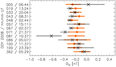
As discussed above, a comparison of simultaneous Oxf values resulting from the SW method and from the TOF or BD methods is impossible due to the complementarity of the methods. In the next best case, Oxf values from either the TOF or the BD method are available before and after an Oxf estimate by the SW method within a common orbit. This is the case for 13 orbits (see dates on the vertical axis of figure 7). Spin axis offset corrections were obtained by the TOF method during both outbound and inbound passes of Cluster 3 through the magnetosphere on those orbits. SW method Oxf values are based on the solar wind intervals in between, around apogees. For each of those orbits, we linearly interpolate TOF method Oxf values and error bounds (Oxf + ΔOxf+ and Oxf − ΔOxf−) to the central times of the solar wind intervals that the SW method has been applied to. The interpolates are shown in figure 7 in red. The corresponding SW method results are depicted in black.
Figure 7. Black crosses and lines: Oxf results from the SW method and corresponding margins of error between Oxf + ΔOxf+ and Oxf − ΔOxf−. Corresponding interpolated TOF method results are depicted by red dots and lines.
Download figure:
Standard image High-resolution image
In eight cases the SW method results are within the margins of error of the TOF method offset corrections (and vice versa). Furthermore, the margins of error overlap in 12 out of 13 cases (exception: DOY 81). The mean Oxf values are −0.23 nT (SW method) and −0.18 nT (TOF method); they are quite similar to the results obtained for the entire year 2008. As can be seen, the TOF method-determined offsets are much more stable; this is reflected in the respective standard deviations of 0.16 nT (SW method) and 0.05 nT (TOF method). The relative stability of the TOF method results suggests that they may be more accurate than the SW method results.
The relative stability of the TOF method results is surprising when taking into account that the TOF method results are based on data from relatively short periods of time (tint = 15 min intervals). The SW method Oxf estimates, instead, are based on solar wind data intervals that are more than one day long. Consequently, we would expect the SW method-based offset corrections to be more time-averaged and, hence, stable than the TOF method results, contrary to our findings.
5. Summary and conclusions
In this paper, we improve the time-of-flight (TOF) method for FGM spin axis offset determination by using a comprehensive error analysis. It allows for the selection of the most accurate offset (correction) estimates Ox for the computations of final spin axis offsets (or offset corrections) Oxf. Furthermore, we introduce a new method for the same task, denoted as beam direction (BD) method, that is complementary to the TOF method. While both are based on the comparison of EDI and simultaneous FGM measurements, the TOF method benefits from low angles ξB and the BD method from low angles ξD. Both conditions are mutually exclusive. Under low magnetic field conditions, the two methods allow for computations of Oxf independently of the ambient magnetic field direction with respect to the spin axis of the observing spacecraft.
In addition, the error analysis enables us to sensibly choose among TOF and BD method results, when both are available. In fact, it facilitates the combination of both methods after their respective steps 2: Ox estimates and the corresponding uncertainties ΔOx may be merged into a single data set. The increased sample size would improve the statistical basis of the final results Oxf or allow for lowering CO and/or increasing C#.
Furthermore, we compare the results of the TOF and BD methods with those from a typically used SW method. These are our findings:
- In general, the offset correction results for the considered Cluster 3 FGM data from 2008, obtained with the three methods, tend to lie consistently around −0.2 nT.
- Standard deviations of the results of either of the three methods are on the order of 0.1 nT. Systematic differences between results from different methods are equal or smaller.
- Errors 〈ΔOxf〉 are typically a little larger, yet very similar among the three methods: around 0.13 nT, on average.
- Oxf values from the TOF or BD methods are mostly included in the error margins of the corresponding Oxf estimates from the respectively other method. This further indicates that the TOF and BD method results are quantitatively very similar.
- The comparison of the TOF and SW method results shows that the latter seem to be less stable, in contrast to expectations. This finding suggests (without proof) that the TOF method results are more accurate than the SW method ones.
Altogether, we find the TOF and BD methods to perform similarly well, while the SW method results may be equally or slightly less accurate. Furthermore, the TOF and BD methods are able to provide Oxf estimates with much higher cadence (we used tint = 15 min). Instead, the SW method requires solar wind data intervals that are at least several hours long [13]. On the other hand, the TOF and BD methods rely more than the SW method on the accurate knowledge of calibration parameters other than the spin axis offset.
Finally, we approach the question of how readily usable the TOF and BD methods are for routine FGM spin axis offset calibration, in reference to the upcoming MMS mission. We find that most accurate offset estimates are obtained from EDI and FGM measurements in low magnetic field regions. Magnetospheric field strengths per orbit observed by MMS are expected to be highest in the subsolar region. There, field strengths of  nT are typical, just Earthward of the magnetopause. Even under these (worst case) conditions, accurate Ox estimates can be provided at least by the TOF method, likely also by the BD method over a wide range of angles ξB and ξD (see figures 2 and 4). Furthermore, we find that both methods are able to yield Oxf values with (the required) accuracies of 〈ΔOxf〉 ⩽ 0.1 nT or 0.2 nT. Offsets (or, more precisely, offset corrections) fulfilling the latter condition are distributed over almost all orbits for which EDI measurements in low magnetic field regions are available. Hence, we can conclude that the TOF and BD methods, introduced herein, constitute working EDI-based methods that are suitable for routine FGM spin axis offset calibration. This applies in particular to the MMS flux-gate magnetometers, but is dependent on the precise knowledge of the other calibration parameters.
Acknowledgments
We thank the Cluster Active Archive (CAA) team and, in particular, C Carr and R Torbert for the use of Cluster FGM, EDI, and supplementary data. Furthermore, we thank K-H Glassmeier and K-H Fornaçon for the use of Cluster FGM daily calibration files and pertaining FGM data processing software, as well as for valuable discussions on the process of generation and accuracy of the daily calibration files. This research was partly supported by the Austrian Science Fund (FWF): I429-N16.