

Abstract
We use the dielectric continuum model to obtain the polar (Fuchs–Kliewer like) interface vibration modes of toroids made of ionic materials either embedded in a different material or in vacuum, with applications to nanotoroids specially in mind. We report the frequencies of these modes and describe the electric potential they produce. We establish the quantum-mechanical Hamiltonian appropriate for their interaction with electric charges. This Hamiltonian can be used to describe the effect of this interaction on different types of charged particles either inside or outside the torus.
Export citation and abstract BibTeX RIS
1. Introduction
It is well established that phonons have a critical impact on the performance of modern electron devices, both in microelectronics and optoelectronics. Indeed, charge-carrier mobilities, saturation velocities, thermalization rates and other related transport properties are influenced by the interaction of these carriers with phonons. In many applications currently under active development, the reduction of the physical dimensions of devices down to 10 nm naturally leads to additional effects due to the spatial confinement of phonon modes. For instance, the International Technology Roadmap for Semiconductors (ITRS) indicates that the driving of nanometer-scale transistors in sub-22 nm technology nodes will involve important thermal dissipation issues [1].
On the one hand, silicon-based microprocessors and memory chips with a line width as small as 20 nm can meet the demand for low-power multifunctional circuits that can process and store massive amounts of heterogeneous data. However, on the other hand, achieving high performance in devices with physical dimensions near the 'deeper nanoscale' regime of 10 nm or beyond is a challenge for existing technologies. It will require not only dimensional scaling using novel structures and processes, but the complementary metal oxide semiconductor (CMOS) approach will require the introduction of non-silicon materials for the channel, in a similar way as high-permittivity materials have been introduced as new gate dielectric media. In that perspective, materials such as III–V binary and ternary alloys (InP, InGaAs), which show charge-carrier mobilities much higher than silicon, are expected to have an important role in the advancement of semiconductor technology [2–5]. These semiconductors, as well as the III-nitrides, the importance of which is rapidly growing, are more or less ionic, so that the interaction of the carriers with optical phonons can be comparable to or even predominant over that with acoustic phonons.
One way to integrate those materials into a silicon-based structure is to selectively grow them in high-aspect ratio trenches made in the Si substrate. The choice of the appropriate ratio and other geometrical factors such as the slope of the side walls, as well as the sequence of materials to be deposited, has to be performed in order to minimize the generation of defects at the various interfaces. One can assume that, in those very small structures, the characteristics of longitudinal optical (LO) phonons are significantly modified compared to the case of bulk materials. For an extensive review of the properties of phonons in nanostructures, the reader is referred to [6].
The purpose of this work is the study of large-wavelength surface or interface optical phonons (Fuchs–Kliewer like phonons [7]) in torus-shaped nanostructures and of their interaction with electric charges. The use of micrometer-scale toroids as optical resonators has been investigated by several authors. See, e.g. [8, 9]. Obviously, the ring shape of the toroidal systems used by these authors plays a crucial role in producing ultra-sharp resonances. Whether optical phonons or electrons enjoy similar properties in nanotoroids is an interesting and important question, central to the present work. Of course, the dimensions relevant to quantum properties of phonons or electrons are in the range of nanometers rather than micrometers.
We devote this article to the study of surface or interface optical phonons in ionic toroidal systems with emphasis on the case of nanometer dimensions. In the case of ionic crystals in vacuum, the optical surface phonons are responsible for the electrical interaction with external charges located at a distance larger than a few crystal lattice parameters. We use the dielectric continuum model throughout the work. For a discussion of this model, the reader is referred to section 7.1 of [6]. As it neglects the change in the ion short-range interactions at the interface, it is unable to predict the frequency of the short-wavelength interface phonons, nor to describe non crystalline semiconducting media [10]. However, it is by any means appropriate to the description of the electric field produced by optical phonons at distances from the interface larger than the lattice parameter, and of the interaction between the surface or the interface and external electric charges.
The article is organized as follows. We introduce the toroidal coordinates and the toroidal harmonics in section 2. The interface modes, symmetric and antisymmetric with respect to reflections on the torus symmetry plane, are then developed in section 3. In section 4, we deal with the Hamiltonian describing the interface modes. In the same section, we give numerical examples applied to a few common more or less ionic semiconductors. The paper is complemented by appendices where details of the calculations can be found.
2. Toroidal harmonics and coordinates
In the framework of the dielectric continuum model, the search for the interface vibrational modes is directly related to the solution of the Laplace equation with boundary conditions on the surface of the body under investigation. The toroidal harmonics are the solutions appropriate to the case of torus-shaped bodies. We refer the reader to [11] for details. These toroidal harmonics are written as functions of the toroidal coordinates. Different notations are used in the literature. We use those of [11] and define the toroidal coordinates, μ, η, and ϕ, by means of the following relations to the Cartesian coordinates
where

and a is an arbitrary scale constant. Figure 1 shows a few curves in the Oxz plane with constant values of either μ or η. The surfaces with μ constant are tori with Oz as symmetry axis. The intersection of each of these tori with the plane Oxz gives a circle the center of which is on the Ox axis at the position  and the radius is
  ; this radius increases with decreasing values of μ. The surfaces with η constant are spheres with their center on the Oz axis. The variable ϕ gives the rotation angle about Oz, the torus axis. The parameter a constitutes a convenient unit of length, so that, from now on, we take a = 1. This corresponds to replacing x/a by x, y/a by y, and z/a by z. If required, physical dimensions are easily reintroduced at the end of the calculations. A common practice is to use the notations


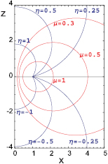
Figure 1. A few curves in the Oxz plane ( ) with either μ or η constant and a = 1.
Download figure:
Standard image High-resolution imageWe adopt this notation, which leads to  .
.
The shape of the circular toroid under investigation is entirely defined by the value  that the toroidal variable μ takes on the torus. The radius of circular sections with axial planes is
  and the distance from the center of these sections to the torus axis is
  . Therefore, the torus major and minor diameters are
  and
and  , respectively. As the geometrical meaning of
  is not readily apparent, it is convenient to introduce characteristic parameters with a more evident meaning. The ratio of the torus major diameter,
  , to its minor diameter, 2Rc, is often used. We prefer to characterize the torus by τ, the ratio of the torus internal diameter (that of the hole around its axis),
  , to its minor diameter, 2Rc. Obviously,

Notice that  entails
  ; this means that, for
  , the central hole of the toroid disappears and the torus touches the toroid axis. The central hole increases in size with respect to the section of the torus for increasing values of
  . Also notice the divergent value of μ (
 ) at
) at  , z = 0, where
  is the distance to the torus axis, and the discontinuity of the variable η across the symmetry plane for
  . Just above the symmetry plane,
  while below it,
  .
.
The following functions

where Tm, n(s) denotes a toroidal harmonic (also called ring function), either

or

constitute complete sets of solutions of the Laplace equation, which is the equation to solve to obtain the interface vibration modes in the dielectric continuum approximation. As usual, the notations P and Q are used for associated Legendre functions of the first and second kind, respectively. Detail of the properties of these functions can be found in a large collection of books and articles. See, e.g. [11–13]. The functions  have a logarithmic singularity at
  and
and  at s = 1. Therefore, the functions Q are convenient to describe the potential inside the torus and the functions P, outside it, at least when no free charges are present. Different definitions of the Legendre functions
  are found in the literature, depending on the branch used in the s complex plane. The reader is referred to appendix A of [13] for a discussion of this point. Here
  is real and
  . Therefore, we choose the definition such that the cut in
  is on the left of s = 1. This is what Mathematica calls type 3 of associated Legendre functions [14, 15].
3. Interface modes
For the sake of completeness, let us briefly recall how the equations obeyed by optical interface phonons with large wavelength are derived in the framework of the dielectric continuum model. Retardation effects are neglected and we restrict ourselves to the case of homogeneous media with isotropic dielectric constants inside as well as outside the torus, which is the case of cubic crystals and most non-crystalline materials. We use Gaussian units throughout the present article. The dielectric constants depend on ω, the electric-field angular frequency. We denote them by  and
and  for inside and outside the torus, respectively. In the absence of free electric charges, the electric displacement obeys
  , with the usual matching conditions of electrostatics at the interface. As
  , with either
  or
or  , the phonon modes are given by
  ,
,  , or
, or  with
with  . The solutions with
  do not exist in an infinite medium and correspond to interface phonon states, which we focus on in this article. The other solutions are confined (bulk-like) modes and will be discussed in a forthcoming paper [16]. Neglecting retardation allows to write
  , where
  is the electric potential of the interface modes. It is solution of the Laplace equation
  with the usual matching conditions of electrostatics at the interface. All this has been discussed in detail by several authors for different sample geometries. See, e.g. [17–19]. Also, see [6] for a more general discussion on phonons in nanostructures.
To obtain the normal modes in the case of toroidal systems, we expand the electric potential in the basis of the functions defined by equations (5)–(7). The matching conditions apply to each  component separately so that a normal mode is characterized by a single value of m. Due to the factor
  in equation (5), this is not true for n and the electric potential of the normal modes is given by a Fourier expansion in
  or
or  . The plane Oxy is a symmetry plane for the torus; the reflection on this plane changes η into
  . Therefore, there are two types of interface normal modes, which are either symmetric or antisymmetric with respect to the reflection on this plane. The electric potential of the symmetric modes contains terms in
  only and that of the antisymmetric ones, terms in
  .
.
The matching conditions of the electric field and displacement on the toroidal boundary lead to sets of linear homogeneous equations in the expansion coefficients. For solutions to exist, the determinant of the equation coefficients must be zero. This constitutes a secular equation in  which gives the spectrum of the optical interface modes. This spectrum consists of discrete series of allowed values of
  ,
,  . We label the solutions of the secular equation with two indices, m, the order of the toroidal function, and l, that of the secular-equation solution. The eigenvalues of symmetric solutions differ from that of antisymmetric solutions so that the solution symmetry should also be specified. All the eigenvalues
  are functions of τ, the parameter defining the shape of the torus, only. They depend neither on the materials constituting the system nor on its size. The dependence on a single parameter allows a general discussion of the interface modes without reference to specific materials. Of course, the numerical calculation of the frequencies, as well as the description of the polarization, requires the knowledge of the dielectric constants on both sides of the torus.
In this article, we report the results concerning the electric field and potential in the case of two torus shapes, a toroid with a small central hole,  , and a toroid with a medium-size central hole,
  . Some details of the calculations are given in appendix
  tend towards −1 for increasing values of τ. Indeed, the limit
  with m finite corresponds to the case of an infinite circular cylinder with an electric potential invariant under translations along the cylinder axis. Then, in cylindrical coordinates, ρ, θ, ζ, and using the cylinder radius as unit of length, the solutions of Laplace equation independent of ζ are
  or
or  inside torus and
  or
or  outside it. The matching conditions for these solutions reduce to
  whatever the value of n. Of course, the degeneracy found in the case of the cylinder is lifted by the curvature of the axis which comes into play when going from the cylinder to the torus.
3.1. Modes symmetric with respect to reflection on torus symmetry plane
Figure 2 illustrates the relation between the eigenvalues  and the shape parameter τ for 5 symmetric modes with l = 1, 2, or 3 and m = 0 or 1.

Figure 2. Eigenvalues  versus τ for 5 symmetric modes with l = 1, 2, or 3 and m = 0 or 1.
Download figure:
Standard image High-resolution image3.1.1. Axisymmetric modes (m = 0).
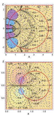
These modes are characterized by m = 0. They are invariant with respect to rotations about the torus axis. Figure 3 gives contour maps of the electric potential in the Oxz plane, with streaming plots of the electric field superimposed on them, in the case of l = 1 phonons with either a small central hole ( ) or a medium-sized one (
 ) while figure 4 gives a three-dimensional view of the potential in the same plane for the same cases. All the figures of electric potentials and fields in this article are snapshots taken at a given time of the ion oscillation cycle. A striking feature is the strengthening of the electric potential and field in the toroid central region, especially in the case of small τ values, i.e. tori with small central empty space, but even in the case of tori with
  . Of course, the actual value of the electric potential depends on the torus size and on the nature of the materials inside and outside the torus.
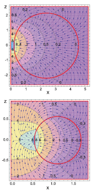
Figure 3. Electric-potential contour maps and electric-field streaming lines in the Oxz plane for m = 0, l = 1 interface phonons; top:  , bottom:
  . The electric potential is in arbitrary units. The circles in red give the intersections of the torus with the Oxz plane and the torus axis coincides with Oz.
Download figure:
Standard image High-resolution image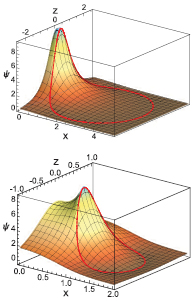
Figure 4. View of the electric potential ψ of m = 0, l =1 symmetric interface phonons in the Oxz axial plane; top:  , bottom:
  . The electric potential is in arbitrary units. The torus axis, Oz, is horizontal. The curves in red give the potential on the intersections of the torus with the Oxz axial plane.
Download figure:
Standard image High-resolution imageIn the case of inside materials with relatively high ionicity, the interaction with virtual m = 0, l = 1 interface phonons could promote the physical adsorption of ions or polar molecules on the axis of torus-shaped nanostructures in contact with gases or liquids. Tori having some similarity to cylindrical holes or pores in thin layers, the interaction with polar interface phonons could strengthen adsorption in these cases too.
The m = 0 phonon modes show a number of peaks in the electric potential increasing with the order l of the eigenvalue  . Some figures are shown on the web page [20]. The oscillatory behavior of the electric potential along the circular intersection with an axial plane can result in weakening the part played by these phonons in the mechanism of adsorption of ions or polar molecules on toroidal nanostructures.
3.1.2. Modes with  .
.

The electric potential of interface modes with  has a spatial oscillatory behavior not only with respect to rotations about the torus axis as expected from the presence of a factor
  or
or  in its expression, but also along the circular intersection with an axial plane. This is exemplified in figure 5, which shows the electric-potential contour map and the electric-field streaming lines for phonons with l = 1 and m =1, in the case of tori with inner circles of radius either small,
  , or medium sized,
  . Notice that, as a result of symmetry, the potential is zero on the torus axis. This fact and the oscillatory behavior of the potential could weaken the role of these phonons in the physical adsorption of charged particles or polar molecules on the torus in the region near its axis. More figures can be seen at URL [20].
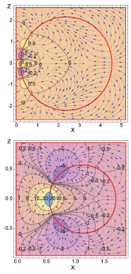
Figure 5. Electric-potential contour maps and electric-field streaming lines in the Oxz plane for m = 1, l = 1 interface phonons; top:  , bottom:
  . The electric potential is in arbitrary units. The circles in red give the intersections of the torus with the Oxz plane and the torus axis coincides with Oz.
Download figure:
Standard image High-resolution image3.2. Modes antisymmetric with respect to reflection on torus symmetry plane
Figure 6 shows the dependence of the eigenvalues  upon τ for 5 antisymmetric modes with l =1, 2, or 3 and m = 0 or 1.
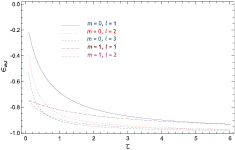
Figure 6. Eigenvalues of  versus τ for 5 antisymmetric modes with l = 1, 2, or 3 and m = 0 or 1.
Download figure:
Standard image High-resolution image3.2.1. Axisymmetric modes (m = 0).
Figure 7 gives contour maps of the electric potential in the Oxz plane, with streaming plots of the electric field superimposed on them, in the case of m = 0, l = 1 antisymmetric phonons with either  or
or  while figure 8 gives a three-dimensional view of the potential in the same plane for the same phonons. Again, the electric potential and field are particularly strong in the toroid central region, especially in the case of small τ values (
 ), but also in the case of intermediate values of τ (
 ). Of course, here also, the actual value of the electric potential depends on the torus size and on the nature of the materials inside and outside the torus. In the case of inside materials that are ionic enough, the interaction with virtual m = 0, l = 1 antisymmetric interface phonons could promote the physical adsorption of polar molecules with their dipole moment lying on the torus axis where the electric field is particularly important.
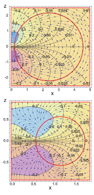
Figure 7. Electric-potential contour maps and electric-field streaming lines in the Oxz plane for m = 0, l = 1 antisymmetric interface phonons; top:  , bottom:
  . The electric potential is in arbitrary units. The circles in red give the intersections of the torus with the Oxz plane and the torus axis coincides with Oz.
Download figure:
Standard image High-resolution image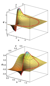
Figure 8. View of the electric potential ψ of m = 0, l = 1 antisymmetric interface phonons in the Oxz axial plane; top:  , bottom:
  . The electric potential is in arbitrary units. The torus axis, Oz, is horizontal. The curves in red give the potential on the intersections of the torus with the Oxz axial plane.
Download figure:
Standard image High-resolution image3.2.2. Modes with .

The shape of the electric potential in the case of non-axisymmetric phonons is illustrated in figure 9, which shows the potential contour map of the m = 1, l = 1 mode. The comparison with figures 7 and 8 shows a significant increase in the number of potential peaks on the torus surface in the vicinity of its central hole, especially if this hole is small. In the case of tori with  , up to 4 maxima and 4 minima can be seen in antisymmetric oscillations with m = 1, while a single maximum and a single minimum are present in the potential of the m = 0 mode. This situation is similar to that of the modes symmetric in respect to the Oxy plane, see sections 3.1.1 and 3.1.2. Here also, the potential is zero on the torus axis, by reason of symmetry. More figures of the electric potential of antisymmetric modes can be seen on the web page [20].
Figure 9. Electric-potential contour maps and electric-field streaming lines in the Oxz plane for m = 1, l = 1 antisymmetric interface phonons; top:  , bottom:
  . The electric potential is in arbitrary units. The circles in red give the intersections of the torus with the Oxz plane and the torus axis coincides with Oz.
Download figure:
Standard image High-resolution image
4. Interface-phonon Hamiltonian
The study of the interaction between interface phonons and electrons (or holes) requires a quantum-mechanical treatment. Therefore we devote this section to the description of the interface phonons and of their interactions with charged particles in the framework of quantum mechanics.
4.1. Derivation of free interface-phonon Hamiltonian
The derivation of the interface-phonon Hamiltonian in the framework of the dielectric continuum model has been described in several papers. See, e.g. chapters 5 and 7 of [6] and the references therein. However, the description is always based on a particular model adapted to a given sample shape and often involves unnecessary lattice sums of dipole interactions. For the sake of completeness and clarity, we describe in this article how the interface-mode Hamiltonian can be derived in the framework of the dielectric continuum model using plain electrostatic theory of dielectrics. The details of the calculations are given in appendix
as expected for a system of harmonic oscillators. In equation (8),  denotes the electric polarization due to the ion oscillations and ω the phonon frequency. The integral is taken over the whole sample volume. The factor
  is
is
In equation (9),  denotes the static dielectric constant,
  , the high-frequency dielectric constant due to the ion electronic polarization alone, and
  , the frequency-dependent dielectric constant measured at the frequency of the polarization oscillations. In the case of interface phonons, the frequency ω is that given by the secular equation,
  . Of course, the values of the dielectric constants are those of the inside or outside medium, depending on the position of the integration point. The contribution of the ion electronic polarizability to the electric polarization is treated in the framework of the usual adiabatic approximation. This means that the energy related to the production of the electronic polarization is not included in the phonon Hamiltonian of equation (8). See appendix
  in the region outside it.
The interface phonons are normal modes of harmonic oscillators with frequencies different from each other and from that of the confined modes. Therefore, they are orthogonal to each other and to the confined modes and the phonon Hamiltonian can be written as a sum of separate Hamiltonians, one for each mode. To obtain the expression of these Hamiltonians, we must replace the electric polarization  in equation (8) by a form appropriate to the mode under consideration. Using
  and
and  shows that the electric polarization of the m, l interface mode is related to the electric potential by
where ψ is the Laplace-equation solution for this m, l mode and  , its angular frequency. The Gauss–Ostrogradsky theorem facilitates transforming the volume integrals into integrals on the torus. Taking the matching conditions at the interface into account and after some calculations detailed in appendix
The index i refers to the torus inside and o to its outside,  is the outward-oriented normal to the torus, and
  is the eigenvalue of the dielectric-constant ratio, solution of the secular equation deduced from the matching conditions. The integral is taken over the torus with surface S. For the sake of conciseness we omit to label the potential with the m, l indices. The notations
  and
and  are used for the values of

measured inside and outside the torus, respectively. Again, if the medium either inside or outside the torus is not ionic, it must be excluded from the energy calculation. Also, recall that there are two types of solutions which are either symmetric or antisymmetric with respect to the Oxy plane.
In section 3 and appendix  inside torus or
  outside it, can be represented in toroidal coordinates by a series of Legendre functions such that

with
for solutions symmetric with respect to the Oxy plane and characterized by the value m of the angular quantum number. In equation (14b),  . The ratios
  are determined by the method described in appendix
  , which gives the amplitude of the oscillation, remains to be determined by the normalization procedure discussed in this section. It has the dimensions of an electric potential while the functions
  and
and  are dimensionless. The normal component of the electric field,
  , is deduced from the derivative of
  with respect to s and the integration involved in equation (11) is performed numerically, taking into account that
  on the torus. Obviously, in the case of symmetric solutions, the phonon total energy is proportional to
  , so that we can write
For the sake of conciseness, we replace the quantum numbers m and l by a single index k. In equation (15),  denotes the interface-phonon frequency and the proportionality factor ck is easily deduced from equation (11), leading to

with
This integral depends on m, l, and τ only. It does not depend on the explicit values of the dielectric constants of the materials that form the system under consideration provided, of course, that they satisfy the secular equation. Table 1 gives its value for  and
and  , and three low-order values of m and l. The reference to specific materials is made through the value of the coefficient in front of
  in equation (16).
Table 1. Value of the integral  for 3 low-order symmetric surface modes.
| m = 0, l = 1 | m = 0, l = 2 | m = 1, l = 1 | |
|---|---|---|---|
 |
299.89 | 1001.7 |  |
 |
387.57 | 2501.5 | 3487.3 |
As  plays the part of a q variable, we write

 being a constant to be determined, qk, the q variable of the interface mode k, and pk, the momentum conjugate to qk. The quantification of the phonon field replaces the variables by operators obeying the usual commutation rules
Introducing the annihilation and creation operators ak and  defined by

and choosing the value of the normalization constant  such that
we obtain
which is the usual form for harmonic oscillators. The parameter  has the dimensions of an electric potential; as for ck, it has that of a length, which is not readily apparent in its definition given by equation (16). This is due to the fact that we took the toroidal-coordinate parameter a equal to 1. Numerical computations require the addition of an extra factor a in the expression of ck.
We treat the case of antisymmetric phonons in a quite similar way. However, the terms in the sum of equation (14) are then in  rather than in
  and the term with n = 0 is absent. Therefore,
  replaces
  in all the equations, starting with equation (13). Finally, this leads to the same form of harmonic-oscillator Hamiltonian, equation (22).
4.2. Interaction with a charged particle
This section is devoted to the study of the interaction of polar interface modes with electrical charges. This type of interaction has been studied in several systems with different geometrical shapes, starting with the pioneering work of Lucas, Kartheuser, and Badro [21] devoted to dielectric slabs. The detailed description of the state of conduction electrons or holes inside the semiconducting toroid and in interaction with the polar phonons lies beyond the scope of the present article. The effects of the interaction with the polar surface or interface phonons on the adsorption of ions and charged molecules or molecular clusters outside the torus is the subject of a forthcoming article [22]. In the present article, we derive and discuss the contribution to the Hamiltonian of the interaction between a point charge and the polar surface or interface phonons in the framework of the dielectric continuum model. Within this approach, the formalism we develop here can, for instance, represent the case of an isolated charge in the neighborhood of a free-standing nanotorus. Completing the Hamiltonian requires the description of the particle, as, e.g. using the band-mass approximation for conduction electrons or holes, that we do not attempt here but leave for a forthcoming publication [16].
Consider a point charge q located at  . In the framework of the dielectric continuum approximation, the electric field acting upon the particle is the macroscopic field
  and the energy of interaction with the mode k is
  inside the torus or
  outside it. Of course, the potential is measured at the charge position. Using equations (13), (14), (18a), and (20a), we obtain

with

inside and outside the torus, respectively. In equation (24), as before,  and η, μ, ϕ denote the toroidal coordinates of the electric charge. It remains to add the Hamiltonian Hq of the free particle, i.e. not interacting with the phonons, and to sum over all the polar surface or interface phonons to obtain the total Hamiltonian
which can be used to describe the state of any type of charged particle in interaction with the phonons under consideration here.
In appendix
4.3. Numerical values of surface-phonon frequencies
For the sake of simplicity, consider the case of a toroid in vacuum or in a gas at moderate pressure. Then  and the interface phonons are simply surface phonons. The secular equation, which gives the frequencies
  , reduces to
  . For the cubic crystals with a single pair of ions per cell studied in the present article, it is a good approximation to take
where  ,
,  , and
, and  are the high-frequency dielectric constant, the frequency of the bulk LO phonons, and that of the bulk transverse optical (TO) phonons, respectively. The former is due to the ion electronic polarizability. The Lyddane–Sachs–Teller relation
straightforwardly deduced from equation (26), relates the static dielectric constant  to these three quantities. Replacing
  by
by  in equation (26) and solving it with respect to
  gives
gives
which determines the surface-phonon frequencies. In equation (28), we have taken into account the fact that the solutions of the secular equation,  , are negative. Clearly,
  entails
  and
and  leads to
  . Therefore, the interface-phonon frequencies lie in the gap between
  and
and  . This well-known result is quite general and not restricted to the case of toroids. The smaller the absolute value of the eigenvalue
  , the closer to
  is the interface-mode frequency. As shown in figures 2 and 6, the absolute value of
  decreases with decreasing values of τ, leading to an increase in the interface-phonon frequencies. This is related to the decrease of the distance between points located on the torus about its axis.
In fact, there is a problem with using equation (28) in the calculation of the surface-phonon frequencies for actual materials, due to the limited accuracy of the known values of the dielectric constants and bulk phonon frequencies. Often, they do not satisfy the Lyddane–Sachs–Teller relation. As the calculated surface-phonon frequencies are close to that of the bulk LO phonons, the error brought by the use of equation (28), while being actually small, has a large effect on the deviation of the surface-phonon frequency from that of the bulk LO modes. Even the sign of this deviation can be wrong, so that the calculated frequencies would appear above the frequency of the bulk LO phonons instead of being in the frequency gap between LO and TO phonons, as they should be. To remedy this situation, the values of  should be derived from
  rather than from
  . This is easily achieved in eliminating
  in favor of
  in equation (28) by means of the Lyddane–Sachs–Teller relation. This results in
This relation has also the advantage of showing why  . Indeed, as
  and, on the other hand,
  as well as
  lie in the range from
  to
to  , an expansion in powers of
  of equation (29) restricted to linear order constitutes a reasonably good approximation. It gives
Consider the case of a toroid made of CdTe, with a large major-radius to minor-radius ratio,  . Then, the difference between
  and
and  can be expected to have a value among the largest possible ones. However, using the numerical values of table 2, we obtain from equation (30)
  , showing that the existence of a surface has not much effect on the polar-phonon frequency. This is due to the small value of the factor
  , 0.043 for CdTe. This reveals the importance of the screening of the ionic polarization by the electronic one.
Table 2. Experimental values of dielectric constants and large-wavelength bulk-phonon frequencies, as well as results of frequency computation, for 3 symmetrical surface phonons in 4 common ionic semiconductors.
| GaAs |
c-GaN |
c-AlN |
CdTe |
||
|---|---|---|---|---|---|
 |
12.8 | 9.7 | 8.07 | 10.2 | |
 |
10.9 | 5.3 | 4.25 | 7.1 | |
 |
33.14 | 68.9 | 80.7 | 17.45 | meV |
 |
35.34 | 91.8 | 111.2 | 20.92 | meV |
 |
|||||
 |
35.31 | 91.25 | 110.35 | 20.86 | meV |
 |
35.26 | 90.54 | 109.25 | 20.78 | meV |
 |
35.18 | 89.26 | 107.30 | 20.62 | meV |
 |
|||||
 |
35.21 | 89.69 | 107.95 | 20.67 | meV |
 |
35.15 | 88.94 | 106.82 | 20.58 | meV |
 |
35.15 | 88.92 | 106.79 | 20.58 | meV |
aMadelung [24].
bDielectric constants: [25]; phonon energies: [26].
cDielectric constants: [27]; phonon energies: [28].
dPerkowitz and Thorland [29]; the value of  is deduced from that of
  using the Lyddane–Sachs–Teller relation.
Table 2 gives the frequencies of some low-index surface phonons in the case of a few more or less ionic cubic semiconductors. The computations have been performed on the basis of equation (29), using the values of the bulk-phonon frequencies and dielectric constants given in the table. As discussed above, the surface-phonon frequencies are always very close to that of the bulk LO phonons.
5. Conclusions
In this article, we describe the polar, Fuchs–Kliewer like modes of interface vibrations of tori made of an ionic material embedded in the bulk of a different substance or simply in vacuum. The presence of an interface does not bring much change to their frequency with respect to that of the bulk large-wavelength LO modes. In a sense, the Fuchs–Kliewer modes constitute the part of the LO modes that produce an electric field outside the body under consideration, i.e. here, the toroid. Even in moderately ionic crystal this field is rather strong, specially on the torus axis and for toroids with a small empty space about the axis. This can lead to a strong interaction with charged or polar particles outside the toroid resulting in modifications of their properties, as for example their optical vibrational spectrum.
Acknowledgments
Financial supports by the project FSRC-13/77 (Université de Liège, Fonds Spéciaux de la Recherche) and the project J.0119.14 (F.R.S-FNRS, Belgium) are gratefully acknowledged.
Appendix A.: Calculation of the interface modes
As discussed in section 3, we write the electric potential of the interface modes symmetric with respect to the Oxy plane as

inside the torus and
outside it. In these equations, the constants  and
and  remain to be determined. Recall that
  and
and  . The antisymmetric modes are obtained from the symmetric ones in replacing the cosine functions in equations (A.1) and (A.2) by sine functions. Of course, the term n = 0 is absent from the expression of the antisymmetric-mode potentials. There also exist solutions in
  but they can be deduced from the present ones by a simple rotation about the torus axis and, therefore, can be discarded.
The matching condition for the ϕ-tangential component of the electric field requires that  , where
  , i.e. the value of the variable s on the toroidal boundary. This results immediately in
so that the electric potential is continuous across the boundary everywhere on the torus, as expected. As a consequence, the matching condition for the η-tangential component of the electric field is also satisfied.
The matching condition for the normal component of the electric displacement is
with

Using equation (A.1), the derivative of the inside potential with respect to s can be written as
The derivative of the outside potential has a similar expression, the Q functions being replaced by P functions and the  coefficients by the
  ones. With these results, the Fourier expansion in
  of equation (A.4) multiplied by
  leads to the following infinite set of homogeneous linear equations coupling
  to
to  and
and  ,
,


with
and, if n > 0,
except for a1, m, which has an extra factor 2,
There exist several methods of solving this type of three-term recursion formula, or tridiagonal system of equations. A straightforward way consists in restricting the system to a finite number N of equations and, then, let N increase progressively. The finite system of N equations has solutions only if the determinant of the coefficient matrix is equal to zero. This leads to a polynomial equation in  , the solutions of which,
  , when solved with respect to ω, give the frequencies of the different interface modes. Of course, this last step requires the knowledge of both dielectric constants, inside and outside the torus. The number of solutions increases with N, the number of equations kept in the calculations. Therefore, seeking higher-order solutions requires to work with a larger number of equations. However, interaction with acoustic phonons and electrons broadens the interface-phonon frequency so that higher-order modes probably overlap and their calculation does not make much sense.
The determinant of a tridiagonal matrix is called a continuant. Continuants can be evaluated by recursion [30], so that the computation of the interface-mode frequencies is relatively simple. It remains to determine the coefficients  from equation (A.7a). However, the recursion is often unstable. A way of avoiding this difficulty consists in transforming equation (A.7a) into a continued fraction. Then, standard stable techniques of computing continued fractions can be used. To obtain a continued fraction, equation (A.7b) is divided by
  , leading to
where  . By successive substitutions, we obtain, in the usual continued-fraction notations,
We use the modified Lentz's method described in, e.g. [31] to compute this continued fraction. We begin with n = 1. The value of  calculated in this way is compared to that given by equation (A.7a) to check the accuracy of the value of
  obtained previously from the zeros of the continuants. In fact, this identification could be used instead of the search for the zeros of the continuants to obtain the characteristic values of
  . The solution of equation (A.12) is repeated for increasing values of n till the contributions to the sum over n in equation (A.1) become negligible.
Appendix B.: Interface-mode potential and kinetic energies
For the reasons discussed in section 4.1, we give here a somewhat detailed account of the derivation of the interface-mode Hamiltonian in the framework of the dielectric continuum model. We restrict ourselves to the case of cubic crystals with two ions per cell. In this case, the contribution of the polarization  to the local electric field
  at the ion equilibrium position is the Lorentz field,
  . From
  we deduce that
 ![$\mathbf{E}=4\pi \mathbf{P}/\left[\epsilon \left(\omega \right)-1\right]$](https://content.cld.iop.org/journals/0953-8984/28/34/345301/revision1/cmaa2badieqn221.gif) . This allows to write
. This allows to write
We use  to denote the frequency-dependent dielectric constant. Of course, the value of this dielectric constant is that relevant to the medium under consideration, either inside or outside the torus. Obviously, the polarization is

where N denotes the number of lattice cells per unit volume, e* the effective charge of the positive ions,  the relative displacement of the positive ions with respect to the negative ones, and α the total polarizability of the crystal cell. Eliminating
  between equations (B.1b) and (B.2) gives
Notice that, in the case of stationary ions ( ), equation (B.3) reduces to the well-known Clausius–Mossotti relation. Assuming harmonic oscillations leads to write

for the equation of motion of the relative displacement  . In this equation, μ is the lattice-cell reduced mass and
  the force constant of the short-range interaction between ions with opposite signs. Using harmonic solutions for
  ,
,  , and
, and  in equation (B.4) and taking equations (B.1b) and (B.3) into account, we obtain the following relation between the oscillation frequency ω and the dielectric constant

with
For the transverse bulk modes  , so that their frequency is the square root of
while for the LO bulk modes  and, therefore, the square of their frequency is
For other values of the frequency ω, either due to free interface oscillations or oscillations forced by an external electric field, solving equation (B.5) with respect to  gives
gives
where
is the high-frequency dielectric constant due to the electronic polarizability of the ions. The Lyddane–Sachs–Teller relation,
where  denotes the static polarizability of the medium under consideration, either inside or outside the torus, results immediately from equation (B.9). Equations (B.7)–(B.9) are well known results; see [6] and references therein. However, they are generally obtained in the framework of studies of particular systems like slabs, cylinders, and quantum dots. The present developments show that they are in fact quite general.
The ion potential energy has two contributions. The first one is related to the short-range interaction. Per unit volume it is
The second one is due to the action of the electric force on the ions. The electric work per unit volume for a change  of the ion relative position is
  . This shows that the ion electric potential energy per unit volume is
We treat the ion electronic polarization in the framework of the usual adiabatic approximation. Its action on the ion motion appears through its contribution to the local electric field which is the source of the ion electric potential energy. Therefore, the contribution of the electronic polarization to the energy is taken into account by equation (B.13). Going beyond the adiabatic approximation would require a second system, excitons or plasmons for example, coupled to the phonons. The free-oscillation frequencies of this system lie at far higher frequency. The energy of interaction between the electric field and the electronic polarization is a function of the variables describing this second system and not of the phonon variables and, therefore, must not be included in the Hamiltonian derived in the present article.
As for the kinetic energy per unit volume, it is
so that the phonon Hamiltonian can be written as
where the integral is taken over the whole volume. This is the form of Hamiltonian expected for harmonic oscillators. The expression of  ,
,
is obtained by means of equations (B.7)–(B.11).
Introducing the electric potential, we write
Let us consider separately the contributions to the Hamiltonian, HK and HU, coming from the kinetic and potential energies, respectively. We have
and
with
We now focus our attention onto interface phonons. Then, the electric potential is solution of the Laplace equation. Therefore, the last term in equations (B.18) and (B.19) is zero. To evaluate the volume integral of the first term, we apply Gauss–Ostrogradsky theorem. For the inside potential, this reduces the integral to the toroidal surface with an outward-oriented normal. As the nanostructure under study is neutral, at large distance, the electric potential decreases at least as r−2 and the electric field as r−3, with increasing r. Therefore, for the outside potential, the integral again reduces to the toroidal surface, but this time with a normal oriented toward torus inside. For the whole system we obtain


where the index i denotes the torus inside, o its outside, and  the outward oriented torus normal. The dielectric constants are related by
  where
where  is the eigenvalue of the dielectric-constant ratio corresponding to the oscillation mode under consideration. The continuity of the potential across the torus and the matching condition of the electric field imply
  and
and  so that
This is equation (11) used in section 4.1 devoted to the derivation of the interface-mode Hamiltonian.
Appendix C.: The case of bulk LO phonons
As a test, we apply the results of appendix B to the case of large-wavelength LO bulk phonons in interaction with charged particles, i.e. that of Fröhlich polarons [23, 32]. The angular frequency of the LO bulk modes,  , is such that
  ; then
We use a procedure similar to that of [32] and expand the polarization into a series of longitudinal plane waves,
The normalization factor in equation (C.2) has been chosen so that the free-phonon energy takes the form of the Hamiltonian of a system of harmonic oscillators. We use V to denote the sample volume used in the development into Fourier series. The polarization being real requires that  . The free-phonon total energy, equation (B.15), becomes
which is the result expected for harmonic oscillators. Notice that, as  ,
,

so that the momentum conjugate to  is
is
and the free-phonon Hamiltonian becomes
Obviously,  .
.
Quantum mechanics requires that the variables  and
and  be replaced by operators obeying the usual commutation rules
 ![$\left[\,{{p}_{\mathbf{k}}},{{q}_{{{\mathbf{k}}^{\prime}}}}\right]=\left(\hslash /i\right){{\delta}_{\mathbf{k},{{\mathbf{k}}^{\prime}}}}$](https://content.cld.iop.org/journals/0953-8984/28/34/345301/revision1/cmaa2badieqn252.gif) . Introducing phonon annihilation and creation operators,
. Introducing phonon annihilation and creation operators,
leads to the usual Hamiltonian of free large-wavelength LO-phonons
The choice of the phase in the definition of  and
and  is custom in Fröhlich polaron theory. Working with complex variables, as we did above, can seem unusual. It is possible instead to use the real and imaginary parts of
  as real variables. This is discussed in detail in [32] and leads to the same final expression for the free-phonon Hamiltonian, equation (C.8).
In the case of LO phonons, the polarization is related to the macroscopic electric potential  by
by
The energy of interaction of a particle of charge − e located at  with the macroscopic electric field due to the LO phonons is
  . Using equations (C.9), (C.2), (C.7a), and (C.1), we finally obtain
This result coincides with that given by Fröhlich [23] in polaron theory. See [32] for more detail. The factor  comes from the adiabatic approximation used to describe the interaction with the crystal electronic polarization. The fact that we recover Fröhlich's Hamiltonian in the case of bulk phonons shows that the role of the electronic polarization is correctly taken into account in the developments of the present article.