
Abstract
The magnetic anisotropy of the ferromagnetic semiconductor (Ga, Mn) (As, P) is studied in a material-specific microscopic k ⋅p approach. We calculate the electronic energy band structure of (Ga, Mn) (As, P) quaternary ferromagnetic alloys using a 40-band k ⋅p model and taking into account the s, p–d exchange interaction and the strain of the (Ga, Mn) (As, P) layer on a GaAs substrate. We determine the variations of the carrier effective masses in the strained (Ga, Mn) (As, P)/GaAs system. The magnetic anisotropy constants obtained from our simulations using a mean-field model are compared with the experimental ones determined by ferromagnetic resonance spectroscopy on a set of samples with constant manganese concentration and varying phosphorus concentration. An excellent quantitative agreement between experiment and theory is found for the uniaxial out-of-plane and cubic in-plane anisotropy parameters.
Export citation and abstract BibTeX RIS
1. Introduction
For the past two decades, research in diluted magnetic semiconductors (SCs) has attracted tremendous interest because of their great potential for different spintronic applied devices [1–3]. Ferromagnetic SCs might combine storage, detection, logic and communication capabilities on a single chip to produce multifunctional devices such as magnetic sensors, spin injectors, and magnetic memories. Among them, the Ga1−xMnxAs compounds have received a lot of attention (see [4] and references therein). These alloys exhibit many interesting magnetic properties, such as a relatively high Curie temperature [5] and complex magnetic anisotropy (MA) that determines the easy magnetization axes in the absence of an external field [6–10]. Since information is stored in the direction of magnetization in magnetic storage devices, switching between several easy axes and precession of the magnetization have been considered for information storage and/or processing [11, 12].
As a consequence of the SC band structure (BS) of Ga1−xMnxAs, the MA is strongly dependent on Mn and carrier concentrations, temperature, and strain [10, 13, 14]. This dependence allows the use of various static or quasi-static methods to intentionally manipulate the magnetic easy axes. The control of the desired direction of the easy magnetization (in-plane or out-of-plane) has been achieved by (i) changing the Mn concentration [6, 15], (ii) changing the carrier concentration by hydrogenation [16], (iii) varying the temperature [6, 17], (iv) choosing different substrates and therefore different growth-induced strain in the magnetic layer [17, 18], (v) bonding the sample to a piezo-transducer and applying a voltage to change the strain [19–21], and (vi) inducing strain relaxation by lithography patterning [12, 22]. Furthermore dynamical modification of the MA by strain was achieved by using short strain pulses to induce a transient change of the MA in order to launch magnetization precession [23, 24].
The prediction of MA under various conditions of strain, Mn and carrier concentrations and its comparison with experimental results has received a lot of attention in Ga1−xMnxAs. Strain control of MA in Ga1−xMnxAs1−yPy, the focus of this paper, has so far been explored much less extensively. Introducing a few per cent of phosphorus at the arsenic sites in Ga1−xMnxAs layers modifies the epitaxial strain continuously from compressive to tensile independently of the Mn doping level [25–27]. One can thereby tune the magnetic easy axis from in-plane to out-of-plane simply by increasing the phosphorus content. Moreover, these layers contain much fewer defects than Ga1−xMnxAs layers designed to produce normal-to-plane magnetic easy axis, such as Ga1−xMnxAs grown on a relaxed (Ga, In)As buffer layer. Indeed, the self-organization of magnetic domains in periodic patterns, impossible to reach in (Ga, Mn)As/(Ga, In)As, was observed in (Ga, Mn)(As, P)/GaAs [28]. These quaternary layers also have other important advantages over Ga1−xMnxAs. For example, it has been predicted that the decrease in the lattice constant of Ga1−xMnxAs1−yPy should lead to an increase in the Curie temperature and the exchange integral Jpd [29], which was partly confirmed by experiments [28].
As far as we know, although several works were devoted to the study of Ga1−xMnxAs1−yPy [25–31], the phosphorus composition dependence of the Ga1−xMnxAs1−yPy band parameters and the link between MA and the BS has not been theoretically investigated. Let us note that one cannot simply map onto Ga1−xMnxAs1−yPy the calculations performed for Ga1−xMnxAs. These generally use the band parameters of GaAs. Here one needs to input the BS of the GaAs1−yPy alloy.
In a recent article [32], we have investigated the effect of epitaxial strain on the MA in a ferromagnetic (Ga, Mn)(As, P) thin film with a typical composition of Mn 7% and P 7%. One of the remaining open questions is the influence of phosphorus fraction on the electronic and magnetic properties of (Ga, Mn)(As, P).
This paper is organized as follows. Section 2 presents the calculation of the energy BS and band parameters of strained Ga1−xMnxAs1−yPy/GaAs within a 40-band k⋅p model using the mean-field Zener model [13]. The influence of subsequent approximations to the electronic structure (6-band k⋅p model) is discussed. The carrier masses and Luttinger parameters are determined as a function of the phosphorus fraction. In section 3, we present a quantitative comparison of the anisotropy parameters obtained from ferromagnetic resonance (FMR) experiments on a set of samples with similar Mn concentration and varying P concentration with our model calculation of the MA using the BS determined in section 2. Section 4 of this work is devoted to the conclusion and perspectives.
2. Band structure
2.1. Methodology
In order to obtain the dependence of the MA as a function of phosphorus fraction, the initial step is the BS calculation of Ga1−xMnxAs1−yPy bulk SCs using k⋅p theory. For this purpose, we use a 40-band k⋅p Hamiltonian first introduced by Saïdi et al [33]. It takes into account the (s, p, d) levels both in the valence bands (VBs) and conduction bands (CBs). We denote by H40 the Hamiltonian matrix. Our 40 × 40 k⋅p Hamiltonian involves matrix elements between the ten  , ten
, ten  , six Γ5C, six Γ5V, two Γ1C, two Γ1V, two Γ1u, and two Γ1q wavefunctions. A full expression of the 40 × 40 Hamiltonian matrix is explicitly given in [34]. This model depends on 10 Γ-centered eigenvalues, 18 spin–orbit coupling coefficients, and 30 matrix elements. In [33], the energy gaps, the momentum matrix elements, and the spin–orbit interaction coefficients used within this model are given in detailed form.
When the crystal is strained, additional terms must be introduced in the k ⋅p Hamiltonian [35–37]. In the case of a biaxially strained Ga1−xMnxAs1−yPy layer grown on a [001]-oriented cubic GaAs buffer, the biaxial strain tensor can be written as a diagonal tensor with elements  xx,yy,zz [10, 13].
In this work, we have adopted the notations of Glunk et al [9] for the relaxed lattice parameter and strain. Hence,  and
and  . The relaxed lattice parameter arel of a biaxially strained layer on a [001]-oriented substrate is given by

where a∥ and a⊥ are the lateral and vertical lattice parameters of the layer. C11 and C12 are elastic stiffness constants of bulk GaAs1−yPy. They are related to the phosphorus content y by (in 1011 dyn cm−2) [38]

Using equation (1), the vertical strain zz can be written as
where  is the lattice mismatch determined by high-resolution x-ray diffraction.
The characteristics of the samples studied in this paper are summarized in table 1. The seven Ga0.93Mn0.07As1−yPy samples are selected in order to compare layers with the same nominal Mn concentration (7%) and different phosphorus concentrations. The samples were grown by low-temperature molecular-beam epitaxy on GaAs(001) substrates. The Mn and P concentrations were calibrated using Vegard's law, based on the lattice constants of a series of GaAs1−yPy references samples grown under the same conditions. After growth, the samples were systematically annealed under nitrogen atmosphere at 250 ° C for 1 h [25]. The data listed in table 1 clearly show that the strain changes from compressive (zz > 0) to tensile (zz < 0) when the phosphorus composition increases in the 50 nm thick Ga1−xMnxAs1−yPy epilayer.
Table 1.
Ga1−xMnxAs1−yPy sample parameters: the phosphorus concentration [P], the lattice mismatch lm, the corresponding strain component zz, the saturation magnetization MS at T = 4 K, the effective Mn concentration xeff, and the splitting parameter of the valence subbands BG.
| Sample | A | B | C | D | E | F | G |
|---|---|---|---|---|---|---|---|
| [P] (%) | 0 | 2.6 | 3.4 | 4.3 | 5.6 | 7 | 11.3 |
| lm (ppm) | 4990 | 280 | 0 | −1200 | −2320 | −3580 | −6620 |
| zz (%) |
0.23 | 0.013 | 0 | −0.055 | −0.11 | −0.16 | −0.31 |
| MS (emu cm−3) | 37.6 | 37.7 | 37.3 | 40.75 | 42.6 | 39.2 | 35 |
| xeff (%) | 3.69 | 3.67 | 3.63 | 3.96 | 4.14 | 3.80 | 3.49 |
| BG (meV) | −26.0 | −26.3 | −26.0 | −28.5 | −30.0 | −27.5 | −24.7 |
The Bir–Pikus HS Hamiltonian matrix used in this work is given explicitly in [34]. Because the influence of strain on p-type CB is unknown, we have taken the p-type CB hydrostatic deformation potential (aΓ5C) and the p-type CB shear deformation potential (bΓ5C) equal to zero. Moreover, we do not use the Bir–Pikus Hamiltonian for the s-type VB, which is at about −12.5 eV from the top of the VB, because (i) no parameters are available for this band and (ii) its influence on the CB and on the VB of interest is very small. Thus, we consider aΓ1V = 0. In the same way there is no need to apply the strain to the d-type VBs and CBs.
The presence of Mn ions in Ga1−xMnxAs1−yPy is taken into account by including the s, p–d exchange interactions. Hence, Hexc = Hpd + Hsd describes the exchange coupling between the localized d-electrons and the delocalized holes (p) and electrons (s). Hpd describes the p–d hybridization, which yields an effective exchange interaction between the hole spin s and the Mn spin S (S = 5/2) carrying a magnetic moment −SgμB, where g is the Landé factor and μB the Bohr magneton. The exchange interaction can be further simplified by the mean-field approximation where the virtual crystal approximation is made [2, 13]. The conduction and valence bands exchange splittings are obtained from the exchange energies N0α and N0β, where N0 is the concentration of cation sites and α and β are the s–d, and p–d exchange integrals, respectively. In order to obtain the values of N0β we assume  and β =− 54.5 meV nm3. arel varies from 5.6661 to 5.6359 Å and N0β from −1.20 to −1.22 eV for y from 0 to 11.3%. Since there is no report concerning experimental or theoretical determination of the s–d exchange energy N0α the value 200 meV, as observed for II–VI diluted magnetic SCs [39], has been adopted in this work. Owing to the presence of Mn atoms in interstitial sites the effective concentration of Mn atoms participating in the ferromagnetism is lower than the total one [40]. xeff is deduced from the low-temperature saturation magnetization MS as xeff = MS/(N0SgμB). Table 1 clearly shows that only about 50% of Mn atoms contribute to the magnetization for all samples, revealing that the incorporation of Mn in interstitial sites is not modified by alloying with phosphorus. One should also note that, in the Zener model, the exchange splitting of the valence subbands BG = AFβMS/6gμB is an important parameter for the BS and the MA. The values used in our calculations are given in table 1. The AF parameter describes the enhancement of spin density of states by the carrier–carrier interactions. The best fit with experimental results is obtained with AF = 1.4 (close to the value 1.2 used in [13]).
According to the k ⋅p effective Hamiltonian theory, the total Hamiltonian H of the system used in this work has the general form: H = Hkp + HS + Hexc. Let us note that we have not taken into account the bandgap renormalization arising from the high density of carriers in the (III–Mn)V compounds since we are interested in MA and not in optical transitions.
2.2. Results
In this section we present and discuss the results of the application of our k ⋅p model to the electronic structure calculations for bulk Ga1−xMnxAs1−yPy SC. All these calculations were carried out at the relaxed lattice constant. An example of the BS calculated with the full Hamiltonian H for xeff = 0.0369 and y = 0 is shown in figure 1. The electronic BS of this compounds shows features similar to that of bulk GaAs. The band diagram is well reproduced on a width of about 18 eV. The extended k⋅p method is known to be valid up to 6 eV above and 12 eV below the top of the VB in four directions, namely ΓX,ΓL,ΓK and XU.

Figure 1. BS of Ga0.9631Mn0.0369As compound SC along the high-symmetry lines of the first Brillouin zone.
Download figure:
Standard image High-resolution imageOne of the important effects of the strain and exchange is observable in the VB near-Γ region. In figures 2(a)–(c), we show a magnified BS near k = 0, for three different phosphorus fractions (a) y = 0%, (b) y = 3.4%, and (c) y = 11.3%, corresponding to the regime of compressive, zero, and tensile strain, respectively. It is clear that the degeneracy between heavy-holes (HHs) and light-holes (LHs) at the center of the Brillouin zone is lifted. Moreover, the band energies shift evidently near the Γ point, while there is a smaller shift on other VB regions. The influence of the P concentration is mostly evidenced along the [111] direction (figure 2(c)).

Figure 2. Magnified view of the heavy- and light-hole bands and the split-off band in the vicinity of the k = 0 zone center, for samples with three different phosphorus fractions (a) y = 0%, (b) y = 3.4% and (c) y = 11.3%. (d) Comparison of the 40-band (solid line) and 6-band (dashed line) k⋅p models for the y = 0% sample (Ga, Mn)As.
Download figure:
Standard image High-resolution imageGenerally, due to the presence of the strain, the BS of SCs is altered, which changes the lattice constant and reduces the symmetry of the crystal. It also modifies the energy gaps, and lifts degeneracy. The influence of subsequent approximations on the electronic structure is considered. In figure 2(d) we show the comparison of the VB dispersion obtained from the 40-band model (solid line) and that from the 6-band model (dashed line) for the case of Ga0.9631Mn0.0369As over the [001] and [111] directions. This figure shows a satisfactorily agreement between the two models only up to k ∼ 0.1 Å−1 measured from the Γ edge. For a Fermi energy in (Ga, Mn)As up to ≈100 meV the 6-band model is probably sufficient. For higher Fermi energies (doping level above ≈5 1020 cm−3) the deviation of the 6-band k⋅p model BS from the real BS might lead to an inaccurate estimation of the MA. Let us emphasize that, within the 6-band model, one needs to specify the Luttinger parameters in order to take into account the interaction of the VB with the remote bands. This can be achieved for (Ga, Mn)As by taking the parameters of GaAs, but these parameters are not available for (Ga, Mn)(As, P). In the framework of the 40-band model the coupling between bands is described in terms of the matrix elements and band edges, which are deduced from the experiments. Once the BS is well reproduced with the 40-band model, we then calculate the Luttinger parameters [33] which can be used within the 6-band model. This is an important advantage of the 40-band model compared to the 6-band model.
To investigate the effect of phosphorus fraction on the electronic properties of alloys, we also performed calculations of energy gaps at high-symmetry points in the Brillouin zone. The bandgap energy at Γ point,  , is defined as the difference between the lowest conduction band and the highest VB in the presence of strain and exchange. The variation of
  as a function of the phosphorus content in the quaternary alloy layers Ga1−xMnxAs1−yPy/GaAs is displayed in figure 3. This variation results from four contributions: (i) the increase of the gap of the bulk Ga(As, P) with P concentration (alloying effect), (ii) the down-shift of the gap resulting from the exchange splitting of the valence and conduction bands (almost constant here since N0β and xeff have small variations with y), (iii) the effect of the hydrostatic part of the strain, which increases the gap for compressive strain and decreases it for the tensile one, thus opposing the alloying effect, and finally (iv) the effect of the biaxial strain on the VB, which gives a variation similar to the hydrostatic component but with a smaller amplitude. The increase in the gap seen in figure 3 results from the alloying effect (i). The plateau near y ≈ 4% results from the cancellation of strain contributions (iii) and (iv) at zero strain together with a slightly increased exchange down-shift (13% larger for y = 6% than for 0% and 11.3%).

Figure 3. Calculated bandgap energy  of Ga1−xMnxAs1−yPy as a function of y content for the samples of table 1.
Download figure:
Standard image High-resolution imageWe proceed to understand the role of phosphorus fraction on the effective masses and Luttinger parameters. For that purpose we calculate the effective masses for the s-type CB (me(Γ6C)) and for p-type VBs (mhh,mlh) using the total Hamiltonian H. me(Γ6C) was obtained from the second derivative of s-type CB energy with respect to the wavevector around the Γ point. As can be seen in figure 4(a), the electron effective mass of quaternary Ga1−xMnxAs1−yPy exhibits a non-monotonous dependence on the phosphorus composition. Indeed, me(Γ6C) increases mildly with decreasing compressive biaxial strain, while it decreases rapidly with tensile strain. This non-monotonous behavior reflects a competition between alloying and strain effects. Let us note that the variation of the Mn composition has no effect on the masses since the exchange splitting does not change the band curvature.
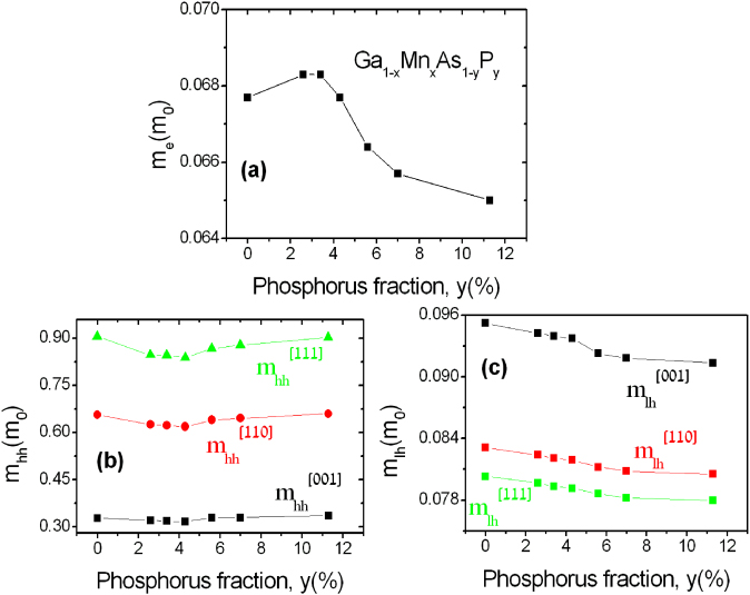
Figure 4. The effective masses of (a) the electron me(Γ6C), (b) heavy-hole and (c) light-hole for Ga1−xMnxAs1−yPy/GaAs calculated using the k⋅p method.
Download figure:
Standard image High-resolution imageGenerally speaking, these observations are consistent with previous experiments and a theoretical study of other bulk SCs [41]. In figures 4(b)–(c), we show the effective masses for both the HH and LH bands along the [001], [110] and [111] directions as a function of phosphorus fraction. mhh and mlh have the same behavior along all three directions. Similarly to the electron mass the HH mass exhibits a non-monotonous behavior with P concentration. It decreases slightly under decreasing compressive strain and increases mildly with tensile strain. The LH mass decreases monotonously with increasing y but the slope of mlh(y) changes when going from compressive to tensile strain. Note finally that the mhh effective mass is the largest along [111] direction, while mlh is the largest along the [001] direction.
An accurate description of the VB effective masses makes our results reliable to calculate the Luttinger parameters γℓ (ℓ = 1–3) from the following expression [42]
and shows that the behavior of the Luttinger parameters is a consequence of the competition between the alloying effect and the strain effect. In figure 5, we show the dependence of the Luttinger parameters on y and compare them to data from the literature for unstrained GaAs1−yPy alloys. The full lines show the y-variation obtained by a linear interpolation between the GaAs and GaP values [43]. The decrease in γℓ (ℓ = 1–3) with increasing y (full lines) can be explained by an important alloying effect. For our calculated values (symbols), the effect of strain differs depending on the regime of strain considered. Indeed, comparatively to the unstrained case, the compressive strain leads to a decrease of the Luttinger parameters while the tensile strain leads to an increase of γℓ.
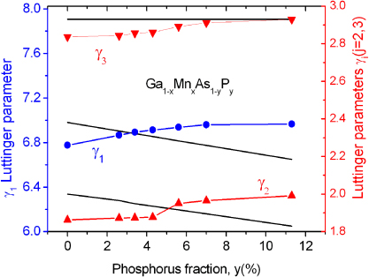
Figure 5. Luttinger parameters γℓ (ℓ = 1–3) of Ga1−xMnxAs1−yPy/GaAs obtained with 40-band k⋅p model (symbols). The full lines represent the Luttinger parameters for unstrained GaAs1−yPy (from [43]).
Download figure:
Standard image High-resolution image3. Magnetic anisotropy
Magnetic anisotropy has attracted much attention because it is essential not only for the fundamental understanding of the microscopic origins of ferromagnetism in diluted magnetic SCs, but also it is of central importance for applications of these materials, since it determines the easy axis of magnetization, the anisotropy fields and the magnetic domain wall width and specific energy. Let us recall that the MA is the dependence of the free-energy density F of a magnetic system on the orientation of the magnetization direction m = (M/M) with respect to the symmetry axes. Recent studies of the ferromagnetic phase in Ga1−xMnxAs1−yPy epilayers demonstrated the existence of rich MA [25, 26, 30]. In order to provide a concise description of the MA, the normalized quantity FM = F/M is considered instead of F. As given in [44–46], there are three contributions to FM: (i) the contribution FM,1(m) that arises from spin–orbit coupling in the VB in a cubic crystal with exchange and biaxial strain, (ii) the contributions FM,2(m) caused by the demagnetization field and a uniaxial in-plane contribution along ![$[1\overline{1}0]$](https://content.cld.iop.org/journals/0953-8984/25/34/346001/revision1/cm469548ieqn165.gif) , whose microscopic origin is still under debate [6, 47–50], and (iii) the contribution FM,3(m) from the single-ion anisotropy [46, 51], which is small and usually neglected. The free-energy functional FM is then given by FM(m) = FM,1(m) + FM,2(m) + FM,3(m). We consider a phenomenological description of the free energy in terms of anisotropy constants and the direction cosines of the magnetization vector mx,my, and mz with respect to the main crystallographic directions 〈100〉. We restrict our calculations to zero temperature and zero magnetic field. In this approximation and taking only up to the fourth-order term for the mi components, the free-energy density for [001]-oriented layers can be written as
, whose microscopic origin is still under debate [6, 47–50], and (iii) the contribution FM,3(m) from the single-ion anisotropy [46, 51], which is small and usually neglected. The free-energy functional FM is then given by FM(m) = FM,1(m) + FM,2(m) + FM,3(m). We consider a phenomenological description of the free energy in terms of anisotropy constants and the direction cosines of the magnetization vector mx,my, and mz with respect to the main crystallographic directions 〈100〉. We restrict our calculations to zero temperature and zero magnetic field. In this approximation and taking only up to the fourth-order term for the mi components, the free-energy density for [001]-oriented layers can be written as
where  . The first three anisotropy components represent contributions to FM,1. The next two contribute to FM,2, and the last three to FM,3. The parameters Bℓ denote the magnetic anisotropy constants.
  is the perpendicular uniaxial anisotropy field resulting from the biaxial strain introduced during the molecular-beam epitaxy growth of GaMnAs layers on substrates with a different lattice constant.
  and
and  are constants representing the in-plane and the perpendicular cubic anisotropy which reflects the non-equivalence of the 〈100〉 and 〈110〉 directions. In the case of a perfect cubic crystal, the symmetry requires B4∥ = B4⊥ and
  . Since growth on a lattice-mismatched substrate introduces tetragonal distortion and breaks the purely cubic symmetry of the crystal lattice, the in-plane and perpendicular cubic anisotropy constants need to be distinguished. Bd is the demagnetizing anisotropy field, arising from shape anisotropy.
  or B2∥ is the in-plane uniaxial anisotropy field that reflects the non-equivalence of
 ![$[1\overline{1}0]$](https://content.cld.iop.org/journals/0953-8984/25/34/346001/revision1/cm469548ieqn189.gif) and [110] directions.
and [110] directions.
In our theoretical approach, we have calculated the FM,1 contribution. The numerical procedure to determine the magnetic anisotropy is described in [9, 32]. Using the BS calculated in section 2, F1 is obtained first by summing over all energy eigenvalues within the four spin-split, HH and LH Fermi surfaces. The resulting energy density is then normalized by the saturation magnetization M. We use the sample parameters specified in table 1. Due to the presence of charge compensating defects depending on growth conditions in Ga1−xMnxAs1−yPy samples, the exact determination of the Fermi level in ferromagnetic Ga1−xMnxAs1−yPy is difficult. Hence, for reasons of simplicity and lack of data on the hole concentration, we have assumed that the Fermi level has a constant value equal to −110 meV from the top of the VB for all samples except sample G. In order to justify this approximation, we calculate the hole concentration ptheo for the chosen Fermi energy, and compare it to the estimated hole concentration pest. The values of pest are obtained by assuming that the reduction of the hole concentration is only due to the presence of interstitial Mn that act as double donors. We have xeff = x − 2xi, where xi is the interstitial Mn content. Consequently, the hole concentration is pest = N0(x − 3xi) = N0(3xeff − x)/2 [52]. The values of ptheo and pest are listed in table 2 for the studied samples. We can see that taking the Fermi level as constant is a fairly reasonable approximation. Let us note that sample G (y = 11.3%) is close to the transition from the metallic to the impurity band conduction regime, as deduced from the temperature dependence of the resistivity. As argued in [2], our model might nevertheless be applicable. Indeed, using a slightly smaller Fermi energy (−81 meV), in agreement with the estimated carrier concentration pest (table 2), we will see that a good agreement between theoretical and experimental MA fields is obtained.
Table 2. Fermi level EF, theoretical carrier density ptheo and estimated carrier density pest of Ga1−xMnxAs1−yPy samples.
| Sample | A | B | C | D | E | F | G |
|---|---|---|---|---|---|---|---|
| EF (meV) | −110 | −110 | −110 | −110 | −110 | −110 | −81 |
| pest (1020 cm−3) | 4.5 | 4.4 | 4.3 | 5.4 | 6.0 | 4.9 | 3.5 |
| ptheo (1020 cm−3) | 4.7 | 3.3 | 3.2 | 4.8 | 6.3 | 4.5 | 3.5 |
In order to compare the microscopic theory with the phenomenological description of the MA, we consider the anisotropic part ΔFM,1 of the FM,1 contribution. When the reference magnetization direction is taken along [100],ΔFM,1 is given by the following expression

For m rotated in the (001) and in the (010) plane, we can write equation (4) as [9]:

and

Once ΔFM,1 is calculated numerically in the microscopic model as a function of the crystalline orientations (θ,φ) for the different phosphorus fractions, the phenomenological description of MA, namely equations (5) and (6), can be fitted to the resulting angular dependences by using B2⊥,B4∥, and B4⊥ as fit parameters.
The results of the microscopic calculations are shown by full symbols in figures 6(a) and (b). The full lines show least-squares fits to the calculated data using equations (5) and (6). We observe that the fit curves are in very good agreement with the microscopic results. This good fit clearly demonstrates that the microscopic theory can be well described by B2⊥,B4∥, and B4⊥. Therefore a realistic description of the FM,1 part of the free energy only needs terms up to the fourth order in m. We proceed to understand the role of the phosphorus fraction on the magnetic properties of Ga1−xMnxAs1−yPy quaternary alloys. For that purpose we calculate ΔFM,1(φ) and ΔFM,1(θ) for three representative P concentrations: y = 11.3% (tensile strain), y = 3.4% (≈ zero strain), and y = 0.0% (compressive strain), respectively. Figure 6(a) shows that in Ga1−xMnxAs1−yPy there is a stronger fourfold cubic in-plane anisotropy constant B4∥ under tensile strain than under compressive strain. Such a behavior has also been shown in the case of Ga1−xMnxAs ferromagnetic SC [9, 53].
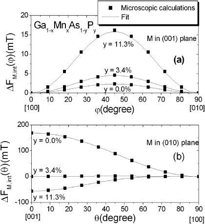
Figure 6. ΔFM,1 calculated as a function of the magnetization orientation and phosphorus concentration for M (a) in the (001) plane and (b) in the (010) plane. The results of the microscopic model are represented by the solid symbols. The solid lines are least-squares fit curves.
Download figure:
Standard image High-resolution imageFrom figure 6(b), we observe that in the regime of tensile strain ΔFM,1 exhibits a minimum for m oriented along [001] (by symmetry also along ![$[0 0\overline{1}]$](https://content.cld.iop.org/journals/0953-8984/25/34/346001/revision1/cm469548ieqn229.gif) ). For compressive strain, the minima occur for m oriented along
). For compressive strain, the minima occur for m oriented along ![$[1 0 0],[\overline{1}0 0]$](https://content.cld.iop.org/journals/0953-8984/25/34/346001/revision1/cm469548ieqn231.gif) , [010], and
, [010], and ![$[0\overline{1}0]$](https://content.cld.iop.org/journals/0953-8984/25/34/346001/revision1/cm469548ieqn233.gif) . Thus, the theoretical model correctly describes the well-known experimental fact that the magnetically hard axis along [001] in compressively strained layers turns into an easy axis in tensile strained layers, as observed in [26]. Note, however, that for the regime of zero strain, the easy axis is not aligned along any high-symmetry direction. This result is due to the values approximately equal taken by the cubic anisotropy parameters (B4∥,B4⊥). These observations clearly point out that the easy axis of magnetization is sensitive to the variation of the phosphorus fraction or, in other words, the preferential axes of the magnetization are closely related to the strain conditions.
. Thus, the theoretical model correctly describes the well-known experimental fact that the magnetically hard axis along [001] in compressively strained layers turns into an easy axis in tensile strained layers, as observed in [26]. Note, however, that for the regime of zero strain, the easy axis is not aligned along any high-symmetry direction. This result is due to the values approximately equal taken by the cubic anisotropy parameters (B4∥,B4⊥). These observations clearly point out that the easy axis of magnetization is sensitive to the variation of the phosphorus fraction or, in other words, the preferential axes of the magnetization are closely related to the strain conditions.
Applying the phenomenological procedure described above to the whole set of Ga1−xMnxAs1−yPy/GaAs layers under study, the anisotropy parameters B2⊥,B4∥, and B4⊥ were determined as a function of phosphorus fraction.
Let us now consider the single-ion anisotropy contribution FM,3. The uniaxial term  can be estimated from the D parameter of the single-ion Hamiltonian used in the analysis of electron paramagnetic resonance experiments (EPR) [46, 51] as
  . Extrapolating the variation of D obtained from EPR for very low Mn concentrations [46] would give
  for Sample A. This is 5% of the value of B2⊥. The
  contribution might even be much smaller since the extrapolation was found to overestimate the D value by a factor of ≈4 for a concentration as low as 0.0027 [51]. The value of D is not known for the same Mn spin state in GaP. However D is proportional to the spin–lattice coupling coefficient G11, which is at least three times smaller in GaP than in GaAs [54]. Therefore we expect that the
  contribution in (Ga, Mn)(As, P) (for the same absolute value of strain) would be even smaller. There might also be a cubic contribution from the single-ion anisotropy. From the a parameter obtained from EPR experiments [46, 51], a
  contribution can be estimated as
  , which amounts to 4 mT. Given the smallness of the single-ion contribution to anisotropy, in the following the experimental results will be compared to the carrier contributions B2⊥,B4∥, and B4⊥.
The experimental magnetic anisotropy constants were obtained by a standard X-band FMR spectroscopy with a 9 GHz microwave source. The angular dependence of the FMR spectra were measured by rotating the static magnetic field in two crystallographic planes: (110) and (001) named 'out-of-plane' and 'in-plane configuration', respectively. These two sets of angular variations of the resonance field enable us to determine the anisotropy constants and associated anisotropy fields [44].
We have taken the experimental data at T = 4.2 K in order to compare with our calculations performed at zero temperature. Firstly, we focus on the behavior of the B2⊥ parameter. In figure 7(a), B2⊥ is plotted versus phosphorus fraction y. The microscopic calculations are in very good agreement with experimental data. However, the results of B2⊥ deduced from the microscopic model are found to be slightly different from the experimental data for y = 3.4% and y = 4.3%. The microscopic model predicts that B2⊥ is linearly proportional to the uniaxial deformation zz. Indeed, a zero value of the uniaxial out-plane parameter is found for zero strain (y = 3.4%). However a non-zero value is obtained experimentally. This discrepancy might originate from the experimental difficulty in determining the strain in this range giving a large error bar at zero strain: ±600 ppm. Additionally, it might be necessary to include higher order terms in FM,1 for the analysis of experimental results when B2⊥,B4∥, and B4⊥ are close to zero. For the range y = 0–7% an almost linear decrease of B2⊥ is evidenced. For larger concentrations 7.0% < y < 11.3%,B2⊥ depends less strongly on y. This result can be explained by the behavior of Luttinger parameters in the range 7.0% < y < 11.3% and the lower Fermi energy for y = 11.3%.

Figure 7. Phosphorus concentration dependence of (a) the uniaxial out-of-plane magnetic anisotropy constant B2⊥, (b) the in-plane cubic anisotropy constant B4∥ and (c) the out-of-plane cubic anisotropy constant B4⊥. The magnetic anisotropy constants obtained with microscopic calculations (circles) are compared with the experimental data obtained from FMR experiments at T = 4.2 K (squares).
Download figure:
Standard image High-resolution image
The fourth-order parameters B4∥ and B4⊥ are presented in figures 7(b) and (c), respectively. We can see that the experimental data of B4∥ are very well reproduced by the microscopic calculations. The B4∥ values obtained using the 40-band k⋅p model in (Ga, Mn)(As, P) are in much better agreement with experimental values than in ternary (Ga, Mn)As using the 6-band k⋅p model [9]. We believe that the more accurate description of the MA originates from a better description of the bands with our 40-band k⋅p model in the range used for the calculation of the MA, in particular from a good determination of the Luttinger parameters. Besides, the assumption that consists in taking the Fermi level as a constant can be considered as relevant because of the almost perfect agreement between experiment and theory.
Unlike the results of B4∥, those of B4⊥ (figure 7(c)) show large variations between the microscopic values and the experimental ones. This discrepancy becomes less important for samples which present close experimental values of B4∥ and B4⊥ (samples B, D, E, and G). However, the predictions of microscopic calculations could not explain the large variation observed in samples A, C and F. Moreover, we can notice that the change of sign for B4⊥ is not reproduced by microscopic calculations. The same problem has also been reported in [9] for Ga1−xMnxAs. At the moment, the reason for this discrepancy is not yet understood. We cannot exclude the possibility that the change of sign of B4⊥ is an artifact of the experimental method for determining B4⊥ [9, 44]. In samples with high B2⊥ coefficient the experimental determination of B4⊥ might be unreliable [10].
4. Conclusion
To summarize, we have presented a theoretical survey of the magnetic properties of ferromagnetic Ga1−xMnxAs1−yPy/GaAs epilayers using the mean-field approximation and the 40-band k⋅p model, in which the BS and band parameters are calculated. The present k⋅p description accurately reproduces the overall band diagram, as well as the band shifts and the carrier effective masses versus phosphorus content. We have considered the effect of the phosphorus composition on the MA. The present microscopic model has been validated through an accurate set of comparisons with experimental results. In particular, the values of B2⊥ and B4∥ anisotropy parameters are very well reproduced.
In the next step, it would be instructive to examine the effect of the introduction of shear deformation in our microscopic calculations. Firstly, the anisotropy coefficient B2∥, which may be associated with magnetostriction or may result from anisotropic Mn distribution [6, 10, 50], plays an important role in the orientation of the in-plane magnetic easy axes. This in-plane uniaxial MA has the same symmetry as the one that would arise from an xy shear strain although never evidenced experimentally. Secondly, the recent demonstration of magnetization precession triggered by quasi-transverse picosecond strain pulses emphasizes the importance of shear deformation for magnetization manipulation [55].
The 40-band k ⋅p model also offers the possibility to calculate the optical properties, in particular the dielectric permittivity and the spectral dependence of the magneto-optical Kerr effect, which is of great importance for the optimization of optical pump–probe experiments and magneto-optical imaging of magnetic domains in these ferromagnetic SCs.
Acknowledgments
The authors thank Laura Thevenard from INSP for useful discussions. This work was performed in the framework of the MANGAS project (ANR 2010-BLANC-0424-02).