
Abstract
For He-like ions, photoabsorption and photoionization cross-sections of 1s2 can differ in the resonance region due to possible resonance radiative decays. This difference increases along isoelectronic sequence. As an example, the 2s2p autoionizing state is considered for different atomic elements (Z = 16, 20, 26). For these elements, we use atomic data computed, without radiative damping, by the R-matrix Breit–Pauli code for 1s2 and 1s2s photoionization processes, which are available on atomic data websites. Applying Davies and Seaton's (1969 J. Phys. B: At. Mol. Phys. 2 757) radiative damping theory, we insert the damping effect. Comparisons are made with similar data computed by another code, which uses Robicheaux et al's (1995 Phys. Rev. A 52 1319) damping theory, also available on an atomic code website. We also present a very simple approximation of Davies and Seaton's theory, and test it by comparisons of data computed with and without the approximation.
Export citation and abstract BibTeX RIS
1. Introduction
Photoionization cross-sections are important to analyse spectra emitted by laboratory or astrophysical plasmas. Many spectroscopic data have already been collected in atomic banks. In particular, the Opacity Project bank [1] contains data derived from close-coupling wavefunctions computed by the non-relativistic R-matrix code [2]. The most important feature, of the close-coupling method, is to give a precise description of collisional resonances, due to autoionization states interacting with continuum, the so-called interference effect or Fano profile [3]. Unfortunately, for highly ionized ions, the resonance lifetime becomes strongly affected by spontaneous emission: there is a competition between autoionization and radiative emission. To include these supplementary effects in the close-coupling formalism, two different approaches have been proposed in the literature called radiative damping theories. The first one, introduced by Davies and Seaton [4], below DS, is based on the traditional time-dependent perturbation theory (e.g. 'Quantum Mechanics' by Bransden and Joachim [5]): close-coupling wavefunctions are not affected by radiation. While, for the second one, proposed by Robicheaux et al, below RGPB [6], an optical imaginary potential is used to insert radiative effects directly in the R-matrix code.
The inverse process to photoionization is photo-recombination. In hot plasmas, recombination is usually more important than photoionization, cold electrons being more abundant than energetic photons. It is traditional to separate photo-recombination data in two non-interfering parts: (i) radiative recombination, corresponding only to the continuum contribution; (ii) dielectronic recombination, corresponding to the autoionizing resonance contribution. To obtain dielectronic recombination data, the most used formalism is time-independent perturbation theory, which includes two perturbations: electron–electron interaction describing autoionization, and radiative interaction describing spontaneous emission. The zero-order Hamiltonian considers autoionizing states as ordinary bound states. Corresponding wavefunctions can be computed by some atomic structure codes. In particular, for He- and Li-like ions, recombination data are essential to study the so-called satellite lines, mainly due to dielectronic recombination [7–9].
In the case of photoionization, only a few initial bound states are important, e.g. ground and metastable levels. While in the case of photo-recombination, the final bound states can be numerous, e.g. large n Rydberg levels. Bell and Seaton [10] proposed a theory to deal with such a situation. It combines DS theory to quantum defect theory [11]. The scattering matrix used in collision theory is transformed to include radiative damping, and is therefore no longer unitary. This method has a further interest, it can be extended easily to include radiative damping for electron excitation processes involving large n [12]. In particular, this method has been used for He-like excitations [13].
The original R-matrix code was non-relativistic [2]. It was well adapted to the first degrees of ionization, where autoionization is important but radiative effects are negligible. Recent versions of the R-matrix code [14] include relativistic effects and can extend the possibilities of the close-coupling wavefunction approach to highly ionized atoms. Autoionization is still very important, but radiative effects become comparable: damping effects should therefore be included, either by DS or RGPB theories. DS theory is apparently more difficult to use: it requires the computation of principal value (PV) integrals containing poles, which might be solved by analytical fitting of computed data [15–17]. RGPB theory turns off the difficulty, but all close-coupling computations have to be restarted from scratch. In this paper, we show that the PV problem is not unsolvable numerically, as long as data have been computed on a fine grid. We also describe a very simple approximation, satisfying the unitarity condition of DS theory, which gives approximate results, but still a lot better than original undamped data. Such approximation does not require any PV integral calculations. It can easily be applied to already published data computed without damping, e.g. [1, 18].
2. Davies and Seaton's damping theory
Davies and Seaton [4] assume that they can generalize the scattering matrix Sscatt, used in electron collision theory, to a 'electron–photon' S matrix, by introducing 'photon channels': the number of incoming particles, either electrons or photons, must be balanced by the number of outcoming particles, i.e. the unitarity of the S matrix. The DS theory cannot be used for bound states because no electron enters or exits, but it can be used for autoionizing levels.
The DS electron–photon S matrix contains four sub-matrices: Sp − p, Sp − e, Se − p, Se − e:

where Sp − p and Se − e are squares, and Sp − e and Se − p are rectangular matrices. Se − p and Sp − p are related to photon absorption followed either by electron or photon emissions. From [15], below STB, equations (2), (3), (6), (7) and using equation (A.8) from the appendix, we obtain
where
In the appendix, De − p is defined, (A.6). In particular, equation (A.9) shows that D†e − p De − p is a real and symmetric matrix. Lp − p is then complex and symmetric, i.e. Lp − p = Ltp − p. In (2.3), the Lp − p matrix can be separated into real and imaginary parts:
The Cauchy principal value integral (PV) can be written as follows:
Due to the fact that the integrand is now continuous, the integral can be carried out numerically. From former equations, DS has proved that the electron–photon S matrix is unitary:

When De − p is small, i.e. Lp − p ≃ 0, the damping effect becomes negligible. One may consider the 'first-order' (i.e. undamped) approximation S(1), from equation (2.2):
S(1) is not a unitary matrix, while the scattering matrix, Sscatt, is. To obtain unitarity (2.6), the simplest method is to replace, in (2.2), Lp − p by its real part:

i.e. to neglect  , Cauchy principal value integrals, (2.5). In the next sections, it will be called the ZD approximation.
3. He-like ion 1s2 photoionization cross-section, near 2s2p 1P1 resonance
The following He-like ions are considered: Fe24 +, Ca18 + and Si14 +. For each of them, two photoionization cross-sections (1s2 and 1s2s 1S0 states) have been computed by Mendoza [19], using the Breit–Pauli R-matrix code (without damping effects) [14], available at http://amdpp.phys.strath.ac.uk/tamoc/codes/serial/asy-damp/.
The 2s2p 1P1 resonance interacts only with a one-electron channel, 1s +  1sp, where 1s is the energy of the photoionized electron and p represents, l = 1. In the same website, a code can also be found to compute photoionization cross-sections with damping effects, using RGPB damping theory. In section 3.1, we consider only photoionization of 1s2s 1S0, i.e. the one-photon channel. In section 3.2, we consider both photoionization processes, i.e. two-photon channels.
The original 'undamped' photoionization cross-sections for 1s2 and 1s2s 1S0 (Q1(ER) and Q2(ER)) are given in Megabarn (1 Mb= 10−18 cm2), and energy ER is in Rydberg (Ryd) (ER = 2E = 21s). They can be converted to area atomic units a20 (a0 = 0.529 18 × 10−8 cm). For simplicity, j = 1 corresponds to 1s2 and j = 2 to 1s2s. Photoionization of 1s2 and 1s2s 1S0 (J' = 0, even) gives only J = 1, odd states, according to the electric dipole selection rule. Using STB (19), we obtain
where α ≃ 1/137 is the fine-structure constant, ωj are photon energies in atomic unit (au): for Fe24 +, ω1 = 1s + 324.84 (au) and ω2 = 1s + 79.5 (au). From (2.4)

The reactance matrix K has only one term, K11, a real number (see the appendix). Defining δ such that K11 = tan δ, it gives, (A.8):
i.e.

where dj is a real (positive or negative) number. Therefore, from (2.4)

Using (3.2), we obtain d21, d22. For a given energy E, we may choose any sign for d1, d2, e.g. both positive, only by changing the sign of 1s or 2s radial functions. For other energies, d1 and d2 being continuous and differentiable functions of E, their signs are defined (see figure 6(a)).
3.1. One-electron channel and one-photon channel
Here, as Sakimoto et al [15], we consider 1s2s 1S0 photoionization for Fe24 +, i.e. the one-photon channel only. It corresponds to j = 2, defined before. For simplicity, we use the following notations :  and
and  .
.
From the undamped photoionization cross-section, we obtain directly  . Using (2.2),
where

Since a2 and b2 are positive numbers, we obtain

which means for the one-photon channel, a 'damped' |Se − p(E)|2 is always smaller than the corresponding 'undamped' |S(1)e − p|2.
As pointed out in [15], the function  , shown in figure 1, has almost a Lorentzian profile. It is possible by fitting
  to an analytical expression to obtain easily
  . From (2.3) we obtain, using a residue theorem,
where Ea = 351.295 27 Ryd and Γa = 0.0094 Ryd.  can be computed directly from (2.5). In figure 2, we present both computed (solid line) and analytical (dashed line) results. One can see that they are almost identical.

Figure 1. Fe24 +:  versus energy ER, obtained directly from undamped cross-sections (3.1). The stars correspond to computed data in RGPB.
Download figure:
Standard image
Figure 2. Fe24 +:  versus energy ER: computed data (solid line) derived from
  using equation (3.7) (dashed line).
Download figure:
Standard imageWe define a damping factor for 1s2s photoionization as follows:  . In figure 3(a), we plot
  (solid line), compared to ZD approximation
  (dashed line), obtained by neglecting b2. At the top, there is no difference between both curves, but differences appear in the wings. To see them better, in figure 3(b), we plot the ratio (1 + a2)2/(1 + a2)2 + b2. The value of ratio is 1, for ER = Ea, and it tends to 1, for the smallest and larger values of ER. In figure 3(b) there are two minima. They appear in figure 4 as two maxima. The separation between two minima is ΔER = 0.015 Ryd. In figure 4, we plot undamped |(S(1)e − p)12|2 and damped |(Se − p)12|2, as well as approximate damped |(S(ZD)e − p)12|2 defined as
The two maxima are separated by ΔER, which requires a photon resolution of ΔER/(2ℏω2) = 3.0× 10⁻⁵. In the case when ion Fe24 + is in a plasma, we must include Doppler broadening: for an ion temperature of 1 keV, ΔER/(2ℏω2) = 3.2× 10⁻⁴: the two maxima are mixed as a broaden single peak. To better estimate differences in figure 4, we compare the following numerical integrals, I, I(1) and I(ZD). They are defined as follows:

We see that I(1)/I = 2.47 and I(1)/I(ZD)=2.25, i.e. ZD approximation includes 9% less damping than the damping expected by DS theory.

Figure 3. Fe24 +: (a) Comparison of damping factors  (solid line) and
  (dashed line); (b) ratio (1 + a2)2/(1 + a2)2 + b2 (solid line).
Download figure:
Standard image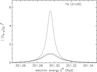
Figure 4. Fe24 +: Comparison of undamped |(S(1)e − p)12|2 (dash–dotted line), damped |(Se − p)12|2 (solid line) and approximate damped |(S(ZD)e − p)12|2 (dashed line)
Download figure:
Standard image3.2. One-electron channel and two-photon channels
We now consider both photoionizations of 1s2 and 1s2s 1S0, i.e. two-photon channels. From (2.2), we obtain
 and
and  have already been presented in figures 1 and 2.
  and
and  curves are plotted in figure 5. For comparison with
  curve (solid line), we also plot the continuum contribution curve (dotted line), represented as a straight line between ER = 351.15 and 351.45 Ryd. By subtracting this contribution from
  , one can estimate the positive and negative contributions of the resonance to photoionization (see later). In figure 6,
  and
and  are plotted. Here,
  changes sign, because d1 has changed sign (
 ). The maxima of
  and
and  are about 1 (figures 1 and 2); the maxima of
  and
and  are about 5.0× 10⁻⁴ (figure 5); and the maxima of
  and
and  are about 2.0× 10⁻² (figure 6). We can use these orders of magnitude to derive the following formula:
where
In figure 7(a), f2 is plotted versus energy ER. We fit it into 0.000 21× a2, and the agreement is excellent. One can rewrite (3.12)

Figure 5. Fe24 + : (a)  (solid line); computed (RGPB) data (stars); continuum contribution (dotted line). (b)
  (solid line) versus energy ER.
Download figure:
Standard image
Figure 6. Fe24 +: (a)  (solid line); numerical calculations (stars). (b)
  (solid line) versus energy ER.
Download figure:
Standard image
Figure 7. Fe24 +: (a) f2 (solid line) and 0.000 21× a2 (stars); (b) c2/(c2 + f2) (solid line) and f2/(c2 + f2) (dashed line).
Download figure:
Standard imageIt is similar to two independent contributions to 1s2 photoionization: (i) c2 contains the direct effect giving the famous Fano profile, and this direct process is independent from 2s2p resonance decaying to 1s2s; (ii) f2 = 0.000 21 × a2, which contains the indirect dependance from 2s2p resonance decaying to 1s2s. Both processes have the same damping factor, i.e.  . In figure 7(b), two ratios are plotted: c2/(c2 + f2) and f2/(c2 + f2). They cross for a ratio = 0.5, the corresponding width is ΔER = 0.013 Ryd, which is smaller than the Doppler width, which is ten times larger. In figure 8, undamped (RPGB) data |(S(1)e − p)11|2, DS damped results |(Se − p)11|2 calculated in this paper and RPGB damped data |(S(RGPB)e − p)11|2 are plotted. We represent RPGB data as stars to distinguish them from DS data (solid line). Also in figure 8, the continuum contribution, |Sc|2, and the ZD approximation, |(S(ZD)e − p)11|2, are shown. The ZD approximation consists of neglecting b2 and f2:
We can compare quantitatively, the importance of the damping process by subtraction of the continuum contribution,|Sc|2 (a straight line, which is tangent to |(S(1)e − p)11|2 at E = 351.15 and 351.45 Ryd), see figure 5. This difference, positive or negative, can be separated into two parts which are integrated separately, but for positive integrand:
where, for example, 2.48( − 5) = 2.48× 10⁻⁵. We see that the integral of the undamped positive part, I(1)+, is strongly decreased by damping, I(1)+/I+ = 2.07, whereas the integral of the undamped negative part, I(1)−, is slightly increased by damping, I(1)−/I− = 0.97. The present approximation (ZD) reproduces well the damping of the positive part I(1)+/I(ZD)+ = 2.02, but overestimates the increase of the negative part I(1)−/I(ZD)− = 0.84. We also see that undamped (I(1)+ − I(1)−) > 0, whereas both (I+ − I−) < 0 and (I(ZD)+ − I(ZD)−) < 0. It means that 1s2 photoionization has been partly destroyed by 2s2p 1P1 resonance, because it decays more to 1s2s than to (1s + 1sp).

Figure 8. Fe24 +: |(S(1)e − p)11|2 (dash–dotted line), |(Se − p)11|2 (solid line), |(S(RGPB)e − p)11|2 (stars), |(S(ZD)e − p)11|2 (dashed line), |Sc|2 (dotted line).
Download figure:
Standard image3.3. Comparison results of RGPB theory and ZD approximation, for S14 +, Ca18 +
As damping effects increase with Z, it is interesting to study other atomic elements of helium isoelectronic sequence. More particularly, it is well known that radiative probabilities depend on Z4, while the autoionization probability stays almost constant. For Fe24 +, radiative damping decreases the photoionization of 1s2s by a factor of 2.5. We expect these decrease effects to be smaller for Ca18 + and even less for Si14 +. For these two He-like ions, we have carried out a similar study to those in subsections 3.1 and 3.2. As for Fe24 +, we find that DS calculations and RGPB data are almost identical. Then, in figures 9 and 10, we compare only RGPB data with ZD data. For Ca (Z = 20) and S (Z = 14), we see only a single peak for 1s2s photoionization. Indeed, the two peaks appear only for |(S(1)e − p)22|2 > 4, i.e. Z ⩾ 24. The difference between RGPB (solid line) and ZD (dashed line) is very small in comparison with undamped results (dash–dotted line). Therefore, most damping effects are taken into account by ZD approximation for photoionization of 1s2s and 1s2. As for Fe24 +, in the case of 1s2 photoionization, we can compare the integrals I+, I−, I(1)+ and I(1)−, after subtraction of the continuum contribution (dotted line). By opposition to Fe24 +, the 2s2p resonance gives a positive contribution, but strongly decreased, compared to undamped ones: Si14 +, (I(1)+ − I(1)−)/(I+ − I−) = 1.96; Ca18 +, (I(1)+ − I(1)−)/(I+ − I−) = 4.54. We also obtain for Si14 +, I(1)+/I+ = 1.21, I(1)−/I− = 0.97; and for Ca18 +, I(1)+/I+ = 1.42, I(1)−/I− = 0.97. The value I(1)−/I− = 0.97 apparently does not change with Z, which means the accuracy is not good enough to be able to see any variation of this quantity.

Figure 9. S16 +: (a) 1s2 photoionization, |Sc|2 (dotted line), |(S(1)e − p)11|2 (dash–dotted line), |(S(RGPB)e − p)11|2 (solid line), |(S(ZD)e − p)11|2 (dashed line); (b) 1s2s photoionization, |(S(1)e − p)22|2 (dash–dotted line), |(S(RGPB)e − p)22|2 (solid line), |(S(ZD)e − p)22|2 (dashed line).
Download figure:
Standard image
Figure 10. Ca18 +: same curves as in figure 9.
Download figure:
Standard image4. Photoabsorption of 1s2 for S, Ca, Fe
Photoabsorption of 1s2 corresponds to the sum of two processes: (i) photoionization (1s2 + ℏω1 → 1s + 1sp), |(Se − p)11|2; (ii) photon transfer (1s2 + ℏω1 → 1s2s + ℏω2), |(Sp − p)21|2.
The first matrix element (i) was already presented, see (3.11). The second one (ii) is a matrix element of Sp − p, defined in (2.2):
Using orders of magnitude, already discussed for (3.11), we obtain
and the ZD expression is
Of course, the undamped value is |(S(1)p − p)21|2 = 0. In figures 11, 12 and 13, results (i) of photon transfer: ω1 → ω2 and results (ii) of photoabsorption by S16 +, Ca20 + and Fe24 + are presented. The continuum contribution |Sc|2 (dotted lines) is given for comparison purpose. For photon transfer, we see that the ZD approximation includes almost 40% of the DS results.

Figure 11. S16 +: (a) |(Sp − p)21|2 (solid line), |(S(ZD)p − p)21|2 (dashed line); (b) 1s2 photoabsorption, |(Se − p)21|2 + |(Sp − p)21|2 (upper solid line); |(Se − p)21|2 (lower solid line) |(S(ZD)e − p)21|2 + |(S(.ZD)p − p)21|2 (dashed line); and |Sc|2 (dotted line).
Download figure:
Standard image
Figure 12. Ca18 +: same curves as in figure 11.
Download figure:
Standard image
Figure 13. Fe24 +: same curves as in figure 11.
Download figure:
Standard image5. Conclusion
In this paper, we try to formulate clearly Davies and Seaton's (DS) radiative damping theory. We applied accurately DS theory to photoionization computations of He-like ions, (Z = 16, 20, 26), near 2s2p 1P1 autoionizing resonance. For Z = 26, we found the same results as those computed using Robicheaux et al damping theory (RGPB). We also present a new approximation (ZD) of DS theory, requiring almost no calculations. The analysis of numerical results shows that ZD approximation has accuracy better than 90% for 1s2s photoionization and slightly less for 1s2. We also compare results obtained by ZD with RGPB damped data for (Z = 16, 20). Finally, we extend DS theory to the calculation of photoabsorption data.
Acknowledgments
The authors thank Dr Claudio Mendoza for helpful discussions and computing undamped and damped photoionization data obtained by RGPB theory.
Appendix:
In the close-coupling approximation, the (N + 1)-electron wavefunctions, ψγ(JE), are projected on N-electron target wavefunctions, coupled to the angular momenta of the projectile electron,  . The projection coefficients are the projectile radial functions. They are solutions of n (coupled) radial equations with real coefficients, with n being the number of channels (called electron channels in this paper), γ''. There are n independent solutions of the total (N + 1)-electron system, γ = 1, ..., n. The total energy is conserved:
  . Solutions of these radial equations can be chosen as either real or complex. The solutions, ψ(K)γ, with real radial functions, satisfy the following asymptotic expression:
where  is called the reactance matrix, (n × n). It is real and symmetric:
  .
.  is the antisymmetrization operator. There are two possible choices for complex radial functions: either the boundary condition corresponds to recombination (incoming electron in channel γ):
or the boundary condition corresponds to photoionization (outgoing electron in channel γ):
where Sscatt is the scattering matrix. It is unitary, symmetric and related to K:
Relations between the solutions Ψ(K), Ψ( + ), Ψ( − ) (row matrices) are
According to STB (4), the definition of De − p (matrix element) is
where  is the photon energy (atomic unit) and α is the fine-structure constant. De − p(Jγ, J'γ'; E) is a complex number only because the radial functions of Ψ( + )γ are complex (phase factor choice). Using instead Ψ(K)γ, we obtain now a real quantity:

Inserting (A.5) in (A.6) and (A.7), we have

and

which is a real and symmetric matrix.