
Abstract
The critical current density of the Nb3Sn superconductor is strongly dependent on the strain applied to the material. In order to investigate this dependence, it is a common practice to measure the critical current of Nb3Sn strands for different values of applied axial strain. In the literature, several models have been proposed to describe these experimental data in the reversible strain region. All these models are capable of fitting the measurement results in the strain region where data are collected, but tend to predict unphysical trends outside the range of data, and especially for large strain values. In this paper we present a model of a new strain function, together with the results obtained by applying the new scaling law on relevant datasets. The data analyzed consisted of the critical current measurements at 4.2 K that were carried out under applied axial strain at Durham University and the University of Geneva on different strand types. With respect to the previous models proposed, the new scaling function does not present problems at large strain values, has a lower number of fitting parameters (only two instead of three or four), and is very stable, so that, starting from few experimental points, it can estimate quite accurately the strand behavior in a strain region where there are no data. A relationship is shown between the proposed strain function and the elastic strain energy, and an analogy is drawn with the exponential form of the McMillan equation for the critical temperature.
Export citation and abstract BibTeX RIS
1. Introduction
Scaling laws describing the electromagnetic behavior of superconductors are essential for the proper design of superconducting devices. Indeed, they allow the full characterization of a superconductor by use of a limited number of experimental results. In addition to temperature and magnetic field, the electromagnetic properties of the Nb3Sn superconductor are strongly dependent on the material's strain. In the reversible strain region, the main parameter describing the Nb3Sn strain dependence is the 'strain' function s(ε). This function is defined as the ratio, at 0 K, between the upper critical field Bc2 of Nb3Sn at a certain strain state ε and its upper critical field at zero strain:
For most of the scaling laws proposed in the literature [1–8, 12, 13], the strain dependence of the superconducting properties can be written as a function of s(ε) as follows:


where w,υ,p and q are parameters that are approximately equal to 3, 1.5, 0.5 and 2 respectively; t ≡ T/Tc(ε) and b ≡ B/Bc2(T,ε).
In order to investigate the strain dependence, it is a common practice to measure the critical current of Nb3Sn strands for different values of applied axial strain εa. In the literature, several scaling laws [1–14] have been proposed for the strain function of the Nb3Sn strand under applied axial strain. All these scaling functions are adequate to fit the measurement results in the strain region where data are available, in a range of strain that can be more or less limited depending on the complexity and number of parameters of the scaling function. However, all the functions tend to predict unphysical trends outside the range of measured data, and in particular for large applied strain values. The reason is that the strain functions do not necessarily converge monotonically to zero for increasing and decreasing applied strain values. Besides the issue of their general asymptotic form, as we show in section 3 of this paper, all the proposed strain functions do not have a sufficient predicting capability in a large strain region: by changing the number of experimental data taken into account in the fit, the parameters and the shape of the strain function can change significantly.
To better describe the reversible high strain region, a new scaling law for the 'strain' function s(ε) has been developed. In this paper the new strain function is presented together with the results obtained by applying the new scaling function to a number of relevant datasets. The data analyzed consist of critical current measurements at 4.2 K that were carried out under applied axial strain at Durham University [15] and at the University of Geneva [16–18] on different strand types. From the critical current measured at a certain applied strain and at various magnetic fields, the Bc2(4.2 K,εa) was calculated using a procedure described in the paper. The Bc2(4.2 K,εa) values were then fit using the proposed strain function.
2. An exponential strain function
2.1. From the original ideas to the final form
In the development of the proposed scaling law, the main assumptions are based on mathematical considerations that take into account the shape of the strain function derived from critical current measurements of strands under applied axial stress. These assumptions can be summarized by the following relationships:

where (1) ε is the strain tensor of the superconductor; (2) F-functions are equal to zero when the argument is zero and positive in all other cases; (3) I1 is the first invariant of the strain tensor, and J2 and J3 the second and third invariants of the deviator strain tensor. The strain tensor represents the global strain status of the material while the deviatoric strain tensor contains only the components producing a variation of shape. Note that equation (5) is equal to one only if the strain tensor is equal to zero; in all other cases, the strain function value is lower than one (and larger than zero).
By approximating the Fi,j functions with a second order Taylor expansion, we then write
where α,β and γ are positive parameters.
The strain function is then further simplified by using considerations related to the form of the three invariants. With respect to the principal strains ε1,ε2,ε3, the three invariants can be written as follows:


By neglecting the terms of fourth order and larger in ε (i.e. J22 and J33) and eliminating the terms that can be negative (I1 and J3 in equation (7), which could lead to exponentials larger than one), the strain function can be simplified to
Equation (11) summarizes the original idea regarding the scaling law proposed in this paper. To specialize the scaling function to the case of uni-axial strain applied to a single wire, we need to introduce further simplifications in the way the variants are evaluated. In this case, it will be assumed that (1) the principal strain component ε1 is along the strand axis (longitudinal component); (2) the other two principal components ε2, ε3, which are perpendicular to the strand axis, are equal. Using these assumptions one can then write


where εa is the axial strain applied to the strand during the measurements; εl0,εt0 are the longitudinal and transverse strains of the Nb3Sn that are due to differential thermal contraction between the Nb3Sn and the other materials of the composite wire; and ν is the 'effective' Poisson ratio of Nb3Sn. The term 'effective' derives from the fact that equations (12) and (13) are the exact solution for the elastic strain of a cylindrical straight beam under pure axial load, but they only represent an approximation for the real strain status of the Nb3Sn filaments. Indeed, the filaments are not straight (they are generally twisted), and they experience not only a longitudinal load but also a transverse one, that is applied by the matrix in which they are embedded.
Finally, by substituting equations (12) and (13) into (8) and (9), one can obtain


From high-energy synchrotron x-ray diffraction measurements on three different types of Nb3Sn wire (bronze route, restacked rod process internal tin, and powder in tube strands) under axial tensile stress at 4.2 K, the effective Poisson ratio of Nb3Sn is estimated to be about 0.36 [19]. Details of the measurement set-up, procedures and data analysis are reported in [20]. A similar value of the effective Poisson ratio was also found by other authors [21] using a similar measurement technique.
Starting from the main ideas presented in the previous paragraphs, equation (11) was then simplified by setting the N value at two in order to limit the number of parameters (N = 1 cannot reproduce the typical asymmetrical shape of the strain function).

When fitting the experimental data with equation (16) and equations (14) and (15) (see section 3 for more information about the analyzed data, and the appendix for tables A.1 and A.2 of the Bc2 data used to derive the optimal parameters of the strain function), it was found that α1 and β2 could be set equal to zero, and hence the strain function was simplified to
C1 and C2 being positive fitting parameters. In order to avoid a second inflection point in the compressive region, the strain function was then slightly modified to
where C3 is a parameter larger than one.
Finally, when deriving the optimal fitting parameters, it was noticed that C2 and C3 could be set equal to constant values that depend on the Nb3Sn 'effective' Poisson ratio. In particular, with an effective Poisson ratio equal to 0.36, C2 and C3 can be set respectively equal to about 1 and 3. Therefore, the strain function assumes the following final form:
In conclusion, assuming an effective Poisson ratio equal to 0.36, the proposed strain function is equation (19), where, in the case of applied axial stress acting on a wire, the invariants J2 and I1 can be calculated using equations (14) and (15). This strain function has originally three fitting parameters C1,εl0 and εt0. Nevertheless, during the calculation of the optimal fitting parameters for the datasets analyzed (see appendix), it was found that εt0 can be written as a function of εl0 in the following way:

where εl0,εt0 are expressed as percentages (as are all the strain values in this paper) and K is equal to 0.1. Hence the fitting parameters are reduced to two: C1 and εl0.
2.2. A relation between the exponential strain function and the elastic energy
Simplifying Nb3Sn as an isotropic linear elastic material, one can write its elastic energy U associated with a strain state ε, as follows [22]:
where v and E are respectively the Poisson ratio and the Young modulus of Nb3Sn. The elastic energy is hence composed of only two terms: one, UI1, associated with the hydrostatic invariant and the other, UJ2, with the second deviatoric invariant. In the case where J2 and I12 values are much smaller or much larger than one, the scaling function (equation (19)) can then be written as
where C1' = 3C1(1 + ν)/E when J2 and I12 are much smaller than one or C1' = C1(1 + ν)/E when the invariants are much larger than one. Assuming an effective Poisson ratio equal to 0.36 as described above, equation (21) becomes

This justifies equation (18), suggesting that the proper quantity for scaling is the elastic energy.
2.3. Analogy between the exponential strain function and the McMillan formula of Tc
The proposed strain function has a form that recalls the formula of the critical temperature developed in the framework of Migdal–Eliashberg theory (which extends the results of BCS theory to the strong coupling regime of the electron–phonon interaction potential [23]):

where λ is the dimensionless electron–phonon coupling constant, measuring the strength of the interaction between electron and phonons in the system, μ* is the renormalized pseudo-potential, recounting the effective strength of the Coulomb repulsion, and 〈ω〉 is the average phonon frequency. Equation (24) is known as McMillan's formula [24, 25], later corrected by Dynes as concerns the multiplicative pre-factor [25, 26]. According to McMillan's formula the critical temperature decreases exponentially to zero on decreasing the electron–phonon coupling constant; on the other hand, from equation (2) and from the proposed strain function, the critical temperature decreases exponentially to zero on increasing the strain in the material. This analogy might suggest that a formulation of the strain function similar to equation (18) might be derived directly from the Migdal–Eliashberg theory once the proper correlation between the electron–phonon coupling constant and the strain is calculated.
2.4. A possible generalization of the exponential strain function
In the proposed exponential function, the strain dependence is ruled by only the two components (hydrostatic and deviatory) of the elastic energy associated with a certain strain. In fact, in equation (19), the dependence of the strain function on one invariant is not affected by the value of the other invariant. This might be a problem in the case of stress loads that modify only one invariant. For example, in the case of increasing pressure the strain function in equation (19) would never go to zero. In order to include this possibility without substantially changing the results discussed so far, one option could be to modify equation (19) as follows:

where C4 is a positive parameter much smaller than C1. Nevertheless, at present the recommended strain function is equation (19).
3. Analysis of relevant datasets
In order to assess the accuracy of the new scaling law, several data sets were analyzed. The data consisted of critical current measurements at 4.2 K that were carried out under applied axial strain at Durham University and the University of Geneva on different strand types. Information about these strands can be found in [15–18].
For each dataset (strand), the upper critical field as a function of the strain was derived from the critical current measurements. The upper critical field as a function of strain was then fit by use of equations (2) and (3) and the proposed exponential scaling law.
3.1. Procedure to determine Bc2(4.2 K, ε)
From the critical current measurements at different magnetic fields and strain, the self-field correction and the pinning force were calculated first. Then, in order to determine the Bc2(4.2 K,ε) values, the experimental data were fit with the following pinning force scaling law:

where C(4.2 K,ε),Bc2(4.2 K,ε),q were free parameters and p was kept constant at 0.5.
During this iterative fit procedure, the critical current data measured at a normalized upper critical field b lower than 0.4 or higher than 0.8 were excluded. Figure 1 shows the results of the fitting procedure for the Furukawa strand tested by Durham University. From the figure one can notice that there are no experimental data in the region around the pinning force maximum (the same was true for all the other datasets analyzed). Because of this and because the p parameter mainly defines the shape of the pinning force in the low field region, p was set equal to 0.5 (that is the value proposed in the Kramer model). In the Bc2 calculation, critical current measurements at normalized fields below 0.4 were excluded to avoid the field region where the pinning force curve might be affected by the use of a non-optimal p parameter. On the other hand, the data at normalized fields above 0.8 were trimmed because at very high field the current can be mostly carried by a limited fraction of the superconductor that has a negligible effect on the transport current properties at lower fields. Indeed, because of composition gradients of Nb3Sn in technical wires, it is known that filaments may contain a relatively small portion of superconducting phase whose upper critical field is higher than the bulk. This portion is generally associated with large grains and composition close to stoichiometry. The fraction of current carried by this superconducting phase is relevant only in the vicinity of Bc2, but decreases to a negligible value for fields significantly lower than Bc2. The effect of non-homogeneous composition is visible in figure 1 as a deviation of the data from the fit at high fields [27, 28].

Figure 1. Pinning force derived from the critical current measurements at 4.2 K of the Furukawa strand. In the plot the black line represent the normalized pinning force as calculated from equation (26) using q equal to 1.41. The different marks represent the experimental data at different applied strain values (in the legend the strain values are represented as percentages).
Download figure:
Standard image High-resolution imageTable 1 summarizes some relevant results obtained from the calculation of the Bc2 for the datasets analyzed. For each strand are reported (1) the calculated q parameter, (2) the number of different values of applied strain at which the tests were performed and (3) the minimum, maximum and average number of critical current measurements used in calculating Bc2 (for different strain values, different numbers of critical current measurements were carried out in the range 0.4 < b < 0.8). Taking the Furukawa wire as an example, 14 different strains were applied, and for a certain εa only five Ic measurements were available for calculating the respective Bc2, while for another εa there were up to 14 Ic measurements. Over the 14 different applied strain values, on average, 10.4 Ic measurements were used to calculate the Bc2.
Table 1. Main parameters in the calculation of Bc2(4.2 K,εa) from the Ic measurements.
| Strand | Type | q | Total number of εa | Number of Ic measurements for calculating each Bc2(4.2 K,εa) | ||
|---|---|---|---|---|---|---|
| Min | Max | Average | ||||
| Furukawa [15] | bronze | 1.41 | 14 | 5 | 14 | 10.4 |
| VAC [15] | bronze | 1.38 | 8 | 8 | 24 | 16.4 |
| OKSC [15] | IT | 1.63 | 10 | 2 | 12 | 7.8 |
| OST [15] | IT | 1.44 | 8 | 2 | 5 | 2.8 |
| PORI [15] | IT | 1.64 | 21 | 4 | 9 | 8.1 |
| UG 8305 [16] | bronze | 1.32 | 28 | 2 | 4 | 3.4 |
| UG 7567 [17] | IT | 1.48 | 29 | 2 | 4 | 3.0 |
| UG 0904 [18] | PIT | 1.91 | 21 | 2 | 6 | 2.8 |
3.2. Fit of Bc2(4.2 K, ε) data using the exponential scaling law
The Bc2 values derived from the eight datasets were fit using equations (2) and (3) and the new exponential scaling law, equation (19). In the calculation, Bc20,C1,εl0 were fitting parameters and Tc0 was set equal to 17 K; note that all the strain values are expressed as percentages (also the invariants refer to the strain as a percentage). Figure 2 shows the results obtained from the strand dataset with the largest range of applied strain [15], while figure 3 shows the exponential strain function derived from the same Bc2 fit with equation (19). In figure 3 the two terms that compose the strain function, the deviatoric and the hydrostatic ones, are also reported. The two components reach their maxima at two different applied strains εD and εH when, respectively, the second deviatoric and the hydrostatic invariants are equal to zero. From equations (14), (15) and (20), one can find that


It is interesting to notice that setting K equal to a constant (in this paper the value 0.1 is recommended) also fixes the difference Δε between εD and εH equal to a constant:

The positive value of Δε together with the different concavities of the two strain function components (see figure 3) is the cause of the typical asymmetric shape of s(ε) with respect to its maximum. Note that, as long as Δε is not zero, the strain function is always lower than one in the case of applied axial strain. Indeed, for any applied strain, there will never be a strain free condition: the hydrostatic and the second deviatoric invariant will never be equal to zero at the same time.
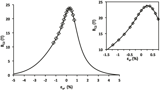
Figure 2. Upper critical field Bc2 at 4.2 K of the Furukawa strand [15] as a function of the applied strain εa: the symbols represent the data derived from the critical current measurements, and the curve the fit obtained by applying the new exponential scaling law.
Download figure:
Standard image High-resolution image
Figure 3. Exponential strain function (continuous line) derived from the fit of the upper critical field at 4.2 K of the Furukawa strand. The dashed lines represent the deviatoric and hydrostatic components (sD and sH) of the strain function (s = sD + sH).
Download figure:
Standard image High-resolution imageFurthermore, from equations (27) and (28) and figure 3, one can also conclude that εl0 establishes the position of εD and εH, and C1 the position of the strain function maximum between εD and εH.
Figure 4 presents a comparison between the different datasets analyzed with their respective fits. In the figure, for the sake of clarity, the Bc2 data were plotted as a function of the difference between the applied strain εa and the applied strain value at which the fitting function has its maximum εMax.

Figure 4. Comparison between the different datasets analyzed. The ordinate axis, which represents the Bc2 in T, have been shifted from one dataset and placed alternately on the left and on the right. The marks show the Bc2 data at 4.2 K while the line shows the fits using the new two parameter exponential scaling law.
Download figure:
Standard image High-resolution imageThe main results of the analysis carried out on the eight datasets are reported in table 2: the upper critical field Bc20; the fitting parameters of the strain function C1 and εl0; the applied strain value εMax where the fitting function has its maximum; the root mean square error between the fit and all the experimental data; and the range of the applied strain where the critical current measurements were carried out.
Table 2. Main parameters calculated by fitting Bc2(4.2 K,ε) with the exponential scaling law.
| Strand | Bc20 (T) | C1 | εl0 (%) | εMax (%) | RMS (T) | Min strain (%) | Max strain (%) |
|---|---|---|---|---|---|---|---|
| Furukawa | 28.67 | 0.901 | −0.29 | 0.28 | 0.05 | −1.22 | 0.73 |
| VAC | 28.80 | 0.958 | −0.30 | 0.29 | 0.14 | −0.73 | 0.73 |
| OKSC | 28.58 | 0.930 | −0.08 | 0.08 | 0.03 | −1.01 | 0.28 |
| OST | 28.39 | 0.875 | −0.10 | 0.09 | 0.12 | −0.97 | 0.29 |
| PORI | 28.24 | 0.869 | −0.09 | 0.08 | 0.14 | −0.92 | 0.31 |
| UG 8305 | 28.84 | 0.643 | −0.28 | 0.28 | 0.05 | −0.05 | 0.77 |
| UG 7567 | 28.62 | 0.752 | −0.25 | 0.25 | 0.04 | −0.34 | 0.47 |
| UG 0904 | 30.97 | 0.735 | −0.18 | 0.18 | 0.06 | −0.63 | 0.34 |
It is interesting to notice that (1) the Bc20 of all the ITER type wires (the first seven in table 2) differ from each other by no more than 0.7 T while the PIT conductor (developed for much higher critical current density [18]) has a significantly higher value as expected; (2) εMax ∼− εl0 (we recall that for an applied strain equal to −εl0 both the deviatoric and the hydrostatic components are not zero; see equations (27) and (28)).
3.3. Stability of the exponential scaling law
Finally, in order to assess the stability of the exponential scaling function compared to previous scaling functions, the root mean square error between the fit and all the experimental data was calculated as a function of the number of experimental data points used for deriving the fit. We considered the strain functions that are most widely used for this task.
The 'Twente' strain function [7]:
where Ca,1,Ca,2,ε0,a and εm are fitting parameters.
The 'Twente modified' strain function [8]:
where Ca,1,Ca,2,ε0,a and εm are fitting parameters. It has been proposed to simplify the 'Twente modified' strain function by using the following relationship to calculate Ca,2 [8]:
which reduces the number of fitting parameters to three.
The 'Markiewicz' strain function [10]:
where C2,C3,C4 and εm are fitting parameters.
The stability analysis was carried out following these steps.
- (1)Define a data window containing a minimum number of Bc2 data points around Bc2 Max.
- (2)By using the pre-defined data window, compute different fits using different scaling functions (figure 5 shows an example for the Furukawa dataset by taking only six points around Bc2 Max).
- (3)Calculate the RMS error between the fitted curve (determined with only a limited number of data points) and the actual data points (all 14 points in the case of the Furukawa dataset).
- (4)The data window (if not containing already all available data) is enlarged by including one more data point, the one closer to the data window, and the calculation restart from step 2.
Tables 3–5 show the fitting parameters of the different scaling functions when applied to the central six points of the Furukawa dataset (see figure 5) and to the whole dataset (14 points).
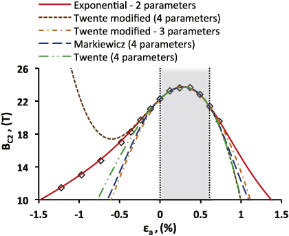
Figure 5. Upper critical field Bc2 as a function of the applied axial strain: diamonds represent the data derived from critical current measurements; the curves shows the fits calculated using only six points around Bc2 Max (those limited by the vertical dashed lines) for different scaling equations.
Download figure:
Standard image High-resolution imageTable 3. Fitting parameters of the exponential scaling function for the Furukawa dataset.
| Number of points | Bc20 (T) | C1 | εl0 (%) |
|---|---|---|---|
| 6 | 28.57 | 0.870 | −0.288 |
| 14 | 28.67 | 0.901 | −0.289 |
Table 4. Fitting parameters of the Twente modified scaling function for the Furukawa dataset.
| Number of points | Twente modified | Twente modified—three parameters | |||||||
|---|---|---|---|---|---|---|---|---|---|
| Bc20 (T) | Ca,1 | Ca,2 | ε0,a (—) | εm (—) | Bc20 (T) | Ca,1 | ε0,a (—) | εm (—) | |
| 6 | 25.30 | 33.55 | 5.56 × 10⁵ | 0.0044 | 2.22 × 10⁻¹⁴ | 25.23 | 62.65 | 0.0097 | 2.23 × 10⁻¹⁴ |
| 14 | 27.06 | 46.29 | 5.08 × 10⁴ | 0.0022 | 0.0026 | 27.08 | 45.52 | 0.002 | 0.0026 |
Table 5. Fitting parameters of the Markiewicz and Twente scaling functions for the Furukawa dataset.
| Number of points | Markiewicz | Twente | ||||||||
|---|---|---|---|---|---|---|---|---|---|---|
| Bc20 (T) | C2 | C3 | C4 | εm (—) | Bc20 (T) | Ca,1 | Ca,2 | ε0,a (—) | εm (—) | |
| 6 | 26.91 | 7.37 × 10³ | 4.53 × 10⁵ | 1.20 × 10⁸ | 0.0029 | 26.92 | 76.69 | 45.82 | 0.0096 | 0.0029 |
| 14 | 26.96 | 8.66 × 10³ | 3.76 × 10⁵ | 5.14 × 10⁶ | 0.0029 | 27.23 | 42.61 | 8.01 | 0.001 | 0.0032 |
Figure 6 summarizes the results obtained using this procedure in the case of the three datasets with the largest range of applied strain. One can notice that the exponential scaling function is the only one that has a reduced RMS value even when using a limited strain range for calculating the fit. This indicates that the fitting parameters of the exponential scaling function are much more stable than those of other scaling functions. Thanks to the improved stability, the exponential scaling function can be used not only as a fitting function, as for the others proposed in the literature, but also for estimating the conductor performance in a strain range where experimental results are not available.

Figure 6. Root mean square error between the Bc2 fit and all the experimental data as a function of the number of experimental data points used for deriving the fit. The more relevant strain functions proposed in the literature were considered for this study. The plots summarize the results for the three datasets with the largest range of applied strain: (a) Furukawa; (b) Vac; (c) OKSC.
Download figure:
Standard image High-resolution image
4. Conclusions
A new scaling law for the strain dependence of Nb3Sn was developed at CERN. It is constituted by the sum of two exponentials whose arguments are respectively functions of the second deviatoric strain invariant and the square of the hydrostatic invariant. In the case of applied axial strain, the strain function has only two fitting parameters, C1 and εl0. This last parameter is the longitudinal pre-strain of Nb3Sn due to the differential thermal contraction between the Nb3Sn and the other wire materials.
In order to assess the accuracy of the new scaling law, eight relevant datasets were analyzed. The data consisted of critical current measurements at 4.2 K that were carried out under applied axial strain at Durham University and the University of Geneva on different strand types. The same datasets were also analyzed by using the more relevant strain scaling functions proposed in the literature. We found remarkably good results from this fitting exercise. Unlike previous proposed models, the new scaling law does not present problems at large strain values, needs a lower number of fitting parameters (only two instead of three or four), and is very stable. This last property is very important to estimate accurately the strand behavior in a strain region where there are no data.
Although we do not show a physical derivation of the scaling function proposed in this paper, we indicate that the proposed strain function has a form that recalls the exponential form of McMillan's formula of the critical temperature developed in the framework of Migdal–Eliashberg theory. This likeness might suggest that a formulation of the strain function similar to the one proposed here might be derived directly from the Migdal–Eliashberg theory once the proper correlation between the electron–phonon coupling constant and the lattice strain is established.
Acknowledgment
The authors would like to thank Dr Jack Ekin for fruitful discussions and useful suggestions while finalizing this paper.
Appendix:
The two tables represent the Bc2 values at 4.2 K that were derived from the critical current measurements measured at Durham University [15] and at the University of Geneva [16–18] on different strand types.
Table A.1. Bc2 values at 4.2 K for the Furukawa, VAC, OKSC and OST strand samples.
| Furukawa | VAC | OKSC | OST | ||||
|---|---|---|---|---|---|---|---|
| Strain (%) | Bc2 (T) | Strain (%) | Bc2 (T) | Strain (%) | Bc2 (T) | Strain (%) | Bc2 (T) |
| 0.73 | 19.54 | 0.73 | 19.29 | 0.278 | 22.65 | 0.29 | 22.71 |
| 0.61 | 21.35 | 0.49 | 23.08 | 0.185 | 23.40 | 0.194 | 23.48 |
| 0.49 | 22.81 | 0.37 | 23.68 | 0.139 | 23.56 | 0.097 | 23.58 |
| 0.37 | 23.63 | 0.24 | 23.55 | 0.093 | 23.66 | 0 | 23.20 |
| 0.24 | 23.59 | 0 | 22.00 | 0.046 | 23.64 | −0.387 | 20.13 |
| 0.12 | 23.23 | −0.24 | 19.37 | 0 | 23.48 | −0.581 | 18.06 |
| 0 | 22.27 | −0.48 | 16.77 | −0.384 | 20.17 | −0.774 | 16.04 |
| −0.12 | 21.04 | −0.73 | 14.62 | −0.592 | 17.82 | −0.968 | 14.19 |
| −0.24 | 19.68 | −0.799 | 15.78 | ||||
| −0.36 | 18.22 | −1.007 | 14.09 | ||||
| −0.48 | 16.98 | ||||||
| −0.73 | 14.77 | ||||||
| −0.97 | 13.01 | ||||||
| −1.22 | 11.46 | ||||||
| 0.73 | 19.54 | ||||||
Table A.2. Bc2 values at 4.2 K for the PORI, UG8305, UG7567 and UG0904 strand samples.
| PORI | UG8305 | UG7567 | UG0904 | ||||
|---|---|---|---|---|---|---|---|
| Strain (%) | Bc2 (T) | Strain (%) | Bc2 (T) | Strain (%) | Bc2 (T) | Strain (%) | Bc2 (T) |
| −0.916 | 14.69 | −0.052 | 22.83 | −0.341 | 19.62 | −0.625 | 19.14 |
| −0.855 | 15.07 | −0.022 | 23.08 | −0.309 | 19.93 | −0.573 | 19.59 |
| −0.794 | 16.00 | 0.009 | 23.28 | −0.278 | 20.30 | −0.521 | 20.12 |
| −0.724 | 16.72 | 0.039 | 23.47 | −0.246 | 20.60 | −0.469 | 20.62 |
| −0.660 | 17.28 | 0.07 | 23.70 | −0.214 | 21.05 | −0.417 | 21.26 |
| −0.611 | 17.67 | 0.101 | 23.84 | −0.183 | 21.33 | −0.365 | 21.83 |
| −0.544 | 18.38 | 0.122 | 23.93 | −0.151 | 21.65 | −0.313 | 22.47 |
| −0.489 | 19.06 | 0.152 | 24.04 | −0.119 | 21.93 | −0.261 | 23.02 |
| −0.428 | 19.79 | 0.182 | 24.12 | −0.087 | 22.19 | −0.209 | 23.56 |
| −0.366 | 20.57 | 0.213 | 24.21 | −0.056 | 22.50 | −0.158 | 24.16 |
| −0.305 | 21.01 | 0.243 | 24.26 | −0.024 | 22.76 | −0.106 | 24.55 |
| −0.244 | 21.50 | 0.277 | 24.35 | −0.003 | 22.96 | −0.054 | 24.90 |
| −0.183 | 22.21 | 0.308 | 24.35 | 0.008 | 22.97 | −0.033 | 25.07 |
| −0.122 | 22.40 | 0.338 | 24.33 | 0.039 | 23.24 | 0 | 25.31 |
| −0.061 | 22.89 | 0.369 | 24.23 | 0.071 | 23.37 | 0.081 | 25.80 |
| 0.000 | 23.23 | 0.4 | 24.11 | 0.103 | 23.59 | 0.19 | 25.97 |
| 0.067 | 23.49 | 0.43 | 23.95 | 0.113 | 23.56 | 0.133 | 25.96 |
| 0.122 | 23.60 | 0.461 | 23.77 | 0.140 | 23.71 | 0.14 | 25.92 |
| 0.189 | 23.34 | 0.491 | 23.54 | 0.175 | 23.83 | 0.162 | 26.03 |
| 0.244 | 22.84 | 0.522 | 23.35 | 0.199 | 23.94 | 0.29 | 25.62 |
| 0.305 | 22.33 | 0.553 | 23.00 | 0.225 | 23.96 | 0.342 | 25.44 |
| 0.583 | 22.74 | 0.256 | 24.04 | ||||
| 0.614 | 22.42 | 0.287 | 23.94 | ||||
| 0.644 | 22.09 | 0.318 | 23.87 | ||||
| 0.675 | 21.61 | 0.350 | 23.78 | ||||
| 0.706 | 21.43 | 0.381 | 23.62 | ||||
| 0.736 | 21.04 | 0.412 | 23.50 | ||||
| 0.767 | 20.65 | 0.443 | 23.13 | ||||
| 0.474 | 22.89 | ||||||