

Abstract
Internal and external flows are characterized by friction factors and drag coefficients, respectively. Their definitions are based on pressure drop and drag force and thus are very different in character. From a thermodynamics point of view in both cases dissipation occurs which can uniformly be related to the entropy generation in the flow field. Therefore we suggest to account for losses in the flow field by friction factors and drag coefficients that are based on the overall entropy generation due to the dissipation in the internal and external flow fields. This second law analysis (SLA) has been applied to internal flows in many studies already. Examples of this flow category are given together with new cases of external flows, also treated by the general SLA-approach.
Export citation and abstract BibTeX RIS
Communicated by K Suga
1. Introduction
One of the most important pieces of information with respect to a flow is that about its losses, i.e. the drag coefficient with external flow around a certain geometry (like an airplane wing) and the friction factor with internal flow through a certain geometry (such as a pipe). Since drag and friction forces act at the surface of the geometry, integrating these tangential and normal forces all over the surface is a straightforward way to determine the drag and the friction forces.
From a thermodynamics point of view, however, these surface forces correspond to the entropy generation in the flow field around and within the geometry under consideration. An inviscid flow with no entropy generation around or within a geometry has zero drag and no friction forces. If, however, entropy generation in the flow field is the volumetric expression of the losses, an integration of this quantity over the flow field will end up with the information about the losses in the flow around or through a certain geometry.
Losses in a flow field are losses of mechanical energy in favor of internal energy. Thermodynamically this is a conversion process between two forms of energy (mechanical and internal) conserving the overall energy (according to the first law of thermodynamics). With the exergy concept (energy = exergy + anergy) this can be expressed as a loss of exergy or available work, corresponding to a devaluation of the energy in the flow field.
When these exergy losses are determined directly from the entropy generation in the flow field, a surface based drag and friction force determination is replaced by one that integrates over the whole flow field. There are several advantages of this approach, which determines exergy losses instead of surface forces.
They are (and will be discussed in the conclusion section):
- (i)a higher accuracy of the final results,
- (ii)detailed information about the location of losses within the flow field,
- (iii)a direct physical interpretation of the losses in terms of exergy losses. This information is not available from drag and friction results since it also depends on the temperature level,
- (iv)a unique assessment quantity for losses in the flow and in the temperature field when heat transfer is also involved.
There is a nice example in favor of the volumetric approach: D'Alambert's paradox in aerodynamics states that the drag is zero when a body is moving in an inviscid fluid. To prove this, one can argue
- (i)surface based: all friction forces at the surface are zero (→ no drag contribution). Pressure forces, however, are not and it remains to be shown that their integral over the whole body is zero. This is not obvious a priori;
- (ii)volume based: if drag would be non-zero, work would have to be done within the flow field (since the point of action moves) and would necessarily change it somehow. Since, however, the flow field is unique (unchanged when the body moves with constant speed) the drag must be zero. This is obvious a priori.
In this study we want to give a comprehensive and unifying presentation of the volume-based approach to determine the losses in a flow field around or through certain geometries.
2. Drag, pressure drop and the second law of thermodynamics
2.1. Conventional loss coefficients
In fluid mechanics external and internal flows are commonly treated as flows that belong to two different categories. When losses are determined for these flows drag is the target quantity for external flows, whereas internal flows are characterized by their pressure drop. In a non-dimensional form they are expressed as drag coefficient cD and friction factor f, which are


Here, D is the drag force on the body, dp/dx is the pressure drop in a conduit, u∞ is the undisturbed oncoming flow and um is the cross section averaged velocity. In order to end up with a non-dimensional cD and f, the projected area A and the hydraulic diameter Dh are included.
Figure 1 shows qualitatively how cD and f look. Here, a Newtonian fluid flows through the pipe (internal flow, characterized by f) and around it (external flow, characterized by cD) as one would anticipate in a shell-and-tube heat exchanger. Both diagrams look roughly similar though in both cases exactly the same physical situation prevails: mechanical energy is converted into internal energy by a dissipation process (accompanied by entropy generation). Therefore, it should be possible to treat both cases consistently.
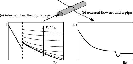
Figure 1. Qualitative shape of the friction factor and drag coefficient curves: (a) internal flow, strong influence of wall roughness ks/Dh, and (b) external flow, no strong influence of wall roughness.
Download figure:
Standard image High-resolution image2.2. Alternative definitions
As an alternative to the conventional definitions cD and f for the drag coefficient and the friction factor, respectively, we suggest to consistently use the entropy generation due to the dissipation of mechanical energy for defining loss coefficients.
For external flows the overall entropy generation rate due to dissipation,  , can be linked to the drag D by considering the (lost) mechanical power PL:

which is a dissipation rate, linked to the entropy generation using the ambient temperature T:

With  from (3) and (4) the drag coefficient cD now is, see equation (1),

For internal flows the pressure drop (− dp/dx) as introduced in equation (2) is a measure for the loss of mechanical energy due to dissipation only for some special (but often occurring) cases. Only when the flow is fully developed and horizontal does (− dp/dx) correspond to the (cross section averaged) dissipation rate. A fully developed flow can occur in pipes and channels only, so that f is no general loss coefficient for internal flows, see Herwig and Schmandt (2012). Its relation to the general head loss coefficient K for internal flows is

since losses obviously are ∝L and ∝1/Dh in pipes and channels.
The lost mechanical power for internal flow again is due to the dissipation process involved, so that a general definition of K is

with φ as the specific dissipation rate in the device in which the internal flow occurs. This dissipation rate is linked to the entropy generation by

so that (7) now becomes

Comparing cD, see equation (5), and this K it turns out that both loss coefficients now are very similar. With  this similarity is even stronger, as can be seen in table 1.
Table 1. Drag and head loss coefficients defined consistently with the entropy generation rate  .
.
| External flow | Internal flow |
|---|---|
 |
 |
| (drag coefficient) | (head loss coefficient) |
| A: projected area | Am: cross section |
| u∞: oncoming flow velocity | um: cross section averaged velocity |
Even though the areas A and Am and the velocities u∞ and um are different in character the combination ϱu3A has a common meaning. It is the real exergy flux for internal flows and for external flows an exergy flux through a fictitious stream tube with the cross section A.
An important aspect of the definitions in table 1 is the occurrence of the temperature T. For isothermal situations at ambient temperature, T is equal to the ambient temperature T∞.
When heat transfer is involved T must be taken as a mean temperature Tm within the flow field. If this Tm is equal to the ambient temperature T∞, cD and K immediately quantify the loss of exergy. If, however, Tm is not equal to T∞ these coefficients are still measure of the dissipation of mechanical energy but no longer a measure of the lost exergy. Since in general according to the so-called Gouy–Stodola theorem, see Herwig and Kautz (2007), the exergy loss is  , the coefficients cD and K must be multiplied by T∞/Tm in order to get a measure for the loss of exergy.
If, for example, on the high temperature level in a steam power plant (Tm = 900 K) dissipation occurs in a pipe, the exergy loss with T∞ = 300 K is only 1/3 of the dissipated mechanical energy and only this part is lost for a conversion into mechanical energy in the turbine.
2.3. Review of literature about entropy generation
The scope of this paper is to provide a comprehensive, unifying definition of loss coefficients for internal as well as external flows. This can be accomplished by relating drag and total head losses to the entropy generation rate in the flow field. Since this  is closely related to the second law of thermodynamics, this approach is called second law analysis (SLA). A literature review with respect to this special aspect should, however, be accompanied by references about entropy in general.
2.3.1. Literature about entropy in general.
There are a vast number of textbooks and monographs about thermodynamics which all have major parts with respect to entropy in it, like Moran and Shapiro (1996), Herwig and Kautz (2007) and Baehr (2009). Special books about entropy range from easy-to-read introductions like Atkins et al (1984), Goldstein and Goldstein (1993) and Dugdale (1996) over more comprehensive books like Falk and Ruppel (1976) and Herwig and Wenterodt (2011) to very challenging ones like Lieb and Yngvason (2000) and Beretta et al (2008).
2.3.2. Literature about entropy generation.
The SLA approach in which irreversibilities are identified and determined is described and applied in fundamental studies like Bejan (1977), Gaggioli (1983) and Sekulic (1986), for example.
Almost all studies that incorporate an SLA refer to one of the several important contributions by Adrian Bejan (1977, 1979, 1982, 1996). In these studies entropy generation is often determined as an integral value within a finite solution domain, either by global balances or by integration of the local entropy generation density. A general and systematic comparison of various approaches can be found in Hesselgreaves (2000) and Herwig and Kock (2007).
As far as internal flows are concerned, one can analyze a system as a whole or have a closer look to single components within a complex system. Studies about whole systems like Anand (1984), Assad (2000) and Nuwayhid et al (2000) aim at improving the system performance, though there is no systematic optimization strategy involved, like in the special study Shiba and Bejan (2001), for example. Detailed studies about single components can be found in Saidi and Yazdi (1999), where a vortex tube is analyzed, in San and Jan (2000) with a study about a crossflow heat exchanger, or in Ko and Ting (2006) where rectangular ducts are investigated, just to mention a few typical investigations out of the big number of studies based on the SLA approach.
In contrast to internal flows the determination of losses by the SLA-approach for external flows is not yet an established method. Therefore, with our study we try to convince the fluid mechanically interested reader that the SLA-approach is at least an attractive alternative to the conventional surface-based way by which drag has so far been determined in a flow field. The role of entropy generation in general is comprehensively discussed in Herwig (2012).
2.3.3. Own literature about the SLA-approach.
In table 2 several papers of our own are listed that cover certain aspects of the SLA-approach for internal flows. They all end up with final results in terms of the head loss coefficient K defined in equation (9), see also table 1, for certain conduit components.
Table 2. Own studies for (incompressible) internal flows.
| Conduit geometry | Flow situation | Reference |
|---|---|---|
| Channel with rough walls | Laminar | Herwig et al (2008a), Gloss and Herwig (2009, 2010) |
| Herwig et al (2010a) | ||
| Pipe, channel with rough walls | Turbulent | Herwig et al (2008b), Herwig and Wenterodt (2010) |
| 90° bend | Laminar | Herwig et al (2010b), Schmandt and Herwig (2011a, 2012), Herwig and Schmandt (2012) |
| (exp. validation Schmandt and Herwig 2012) | ||
| 90° bend combinations | Laminar | Herwig et al (2010b), Schmandt and Herwig (2011a) |
| Stack of sinusoidal plates | Turbulent | Jin and Herwig (2011) |
| 90° bend | Turbulent | Schmandt and Herwig (2011b) |
| 90° bend combinations | Turbulent | Schmandt and Herwig (2011b) |
| Diffusor (optimization) | Turbulent | Schmandt and Herwig (2011c) |
| Pipe flow | Laminar, unsteady | Schmandt and Herwig (2013a) |
| 90° bend | Laminar, unsteady | Schmandt and Herwig (2013a) |
| T-junction | Laminar | Schmandt and Herwig (2013b) |
In the following we will apply the SLA approach in three very different external flow situations, and determine the drag coefficients defined in equation (5), see also table 1. They are the flat plate boundary layer flow (laminar, incompressible), the flow around a sphere (laminar, Re → 0) and the flow around a rising bubble (laminar, Re → 0 and Re → ∞).
Prior to that, details of the SLA will be given in the next section.
3. Details of the SLA-approach
3.1. Determination of 

The pivotal question in the SLA approach is how to determine the local entropy generation rate  in a flow field, the integration of which leads to the (overall) entropy generation
  in equations (5) and (9). When the flow is laminar the determination of
  is straightforward based on the thermodynamics relation (Cartesian coordinates; units: W m−3 K−1; see e.g. Herwig and Kautz 2007):
In order to end up with the overall entropy generation rate  which appears in cD and K, see table 1, this local quantity has to be integrated appropriately. This 'appropriate' integration needs some special considerations when the flow losses of a conduit component in an otherwise fully developed internal flow should be determined, see section 3.2 below.
When the flow is turbulent  according to (10) is adequate only for a direct numerical simulation (DNS)-approach with respect to the turbulence, as for the example shown in Kis and Herwig (2011). Since DNS solutions with their extraordinary computational demand cannot be used for solving technical problems, the time-averaged equations (Reynolds-averaged Navier–Stokes) are solved instead. Then also
  has to be time averaged, so that with
  as time-averaged quantity from now on

with the index  for the entropy generation in the time-averaged velocity field and D' for the time-averaged contribution of the fluctuating parts. Both parts are

With the result for a turbulent flow field from RANS-equations,  according to equation (12) can be determined, but not
  in equation (13). Here, a turbulence model for the fluctuating part
  is needed.
A simple model which basically relates  to the turbulent dissipation rate ε and which can be justified in the limit of infinite Reynolds numbers, see Kock and Herwig (2004), reads

3.2. Determination of for internal flows

Except for the straight pipe or channel, a conduit component has an influence on the upstream and downstream flow within certain upstream and downstream lengths. Within these lengths the influence of the component can be felt by the otherwise fully developed and undisturbed flow. In order to have a clearly defined length of considerable influence upstream and downstream, related lengths Lu and Ld are introduced. They are defined as those lengths up to which 95% of the overall upstream or downstream influence occurs.
Altogether, the situation sketched in figure 2 appears: the central part of the flow field, Vc, being the interior of the conduit component and upstream as well as downstream parts of it, Vu and Vd have to be analyzed with respect to the (additional) entropy generation due to the component. This leads to
In equation (15) referring to figure 2 the overall entropy generation rate is shown to be composed of three parts, the rate within the conduit component and the additional rates upstream and downstream of it. Here,  is the local entropy generation rate of the fully developed and undisturbed flow. Results show that always the upstream influence
  is very small but that the downstream influence
  can be considerable or even be the dominating part in
  , see equation (9).

Figure 2. Determination of the overall entropy generation rate due to a conduit component.  is the additional entropy generation upstream of the component;
  the entropy generation inside the component; and
  the additional entropy generation downstream of the component.
Download figure:
Standard image High-resolution imageIt should be noted that the upstream and downstream parts Vu and Vd have lengths larger than Lu and Ld defined in figure 2. They must be chosen such that the integrals in (15) account for all  with an acceptable truncation error.
3.3. Determination of for external flows

The external flow around a body in a real fluid will always give rise to a drag force. This force has a moving point of action and thus work will be done in the flow field (in contrast to the d'Alembert paradox situation, see section 1 of this paper).
Now that the flow is one of a real fluid with non-zero viscosity, dissipation occurs which is the transfer of mechanical to internal energy. Now the work done by a steadily moving drag force can be found in a permanent increase of the internal energy of the flow field, accompanied by a corresponding entropy generation.
Within the flow field the overall entropy generation rate exactly corresponds to the drag exerted on the body, see equation (5) for cD and table 1. Therefore  in the flow field must be determined, just like for internal flows.
While internal flow fields are unbounded only in the upstream and downstream parts, external flow fields have no direct bounds all around. We define that part of the flow field that has to be taken into account in order to determine  up to a set error as the near flow field. This corresponds to setting certain upstream and downstream lengths in Vu and Vd for internal flows as described in the previous sub-section.
4. Examples
Internal flows have been comprehensively treated by the SLA-approach in the past, see table 2 for a collection of our own studies. Therefore, we just give an example from one of these studies here and concentrate on external flows in the following. For three external flows the drag will be determined by the SLA approach. They are the laminar flow along a flat plate, around a sphere, and around a rising bubble.
4.1. An internal flow example
In figure 3 K-values of a 90° bend with a circular cross section are shown for turbulent flow at various Reynolds numbers taken from Schmandt and Herwig (2011b). The K-value according to equation (9) in figure 3(a) is compared to literature values. In figure 3(b) the cross sectional entropy generation rate  is shown along the centerline coordinate sc. Here the 90° bend lies between sc/Dh = 5 and 5 + π/2. The large area of
  shows that most of the losses occur downstream of the bend. Therefore a K-value does not correspond to the losses in a conduit component but due to it.

Figure 3. K-values of a 90° bend (turbulent flow) determined numerically by the SLA-approach, see Schmandt and Herwig (2011b) and equation (15) for  ,
,  and
and  (a) comparison with literature data, ⊙: Schmandt and Herwig (2011b); +: Ito (1960);
  : Hofmann (1929); –: Idelchik (2007); - -: Miller (1978). (b) Distribution of
  along the centerline coordinate.
Download figure:
Standard image High-resolution image4.2. External flow example 1: flow along a flat plate
Laminar flow over a flat plate of finite length is a benchmark case for the higher order boundary layer theory, described in Van Dyke (1975), for example. This theory is an asymptotic theory for Re → ∞, the results of which can be applied as approximate solutions for finite values of the Reynolds number. Especially when higher order terms are taken into account, the approximation is excellent even for Reynolds numbers of the order  .
.
Such a higher order result for the flat plate of finite length L is

Here the second term on the rhs comes in as the influence of the trailing edge determined by the so-called triple deck theory, see for example Messiter (1983) for more details.
The drag coefficient according to equation (16) will be compared to the results we get from our SLA approach, integrating the local entropy generation in the near flow field. This is done by discretizing the two dimensional steady Navier–Stokes equations with a grid shown in figure 4. There is a grid refinement in the vicinity of the flat plate with details of the grid structure and the numerical solution procedure given in the appendix of this study.

Figure 4. Discretization of the near flow field around the flat plate, plate located between x/lp = 0 and 1.
Download figure:
Standard image High-resolution imageLike in figure 3 for the internal flow example we show the cross section integrated entropy generation rate  along the main stream direction in figure 5, here for the three Reynolds numbers Re = 2, 32 and 512. Comparing the three cases, one can see the increasing boundary layer character for increasing Reynolds numbers: entropy generation (and thus flow losses)occurs more and more in the vicinity of the plate (and in the wake).

Figure 5. Distribution of  along the x-axis, non-dimensionalized with the overall entropy generation rate
  and the length of the plate lp. Location of the flat plate between x/lp = 0 and 1.
Download figure:
Standard image High-resolution imageAt Re = 512 there is almost no upstream influence. Since entropy generation only occurs where velocity gradients are, see equation (10), an almost undisturbed upstream flow field has almost zero  values. Like with internal flows, the entropy generation and thus the losses in the flow field are shifted downstream when the Reynolds number is increased.
Figure 6 shows cD-data determined by the SLA-approach compared to the asymptotic results according to equation (16). Slightly increasing deviations for Re → 0 may be explained by the missing higher order terms  in the asymptotic result in equation (16).

Figure 6. Drag coefficient for the flat plate of finite length lp.
Download figure:
Standard image High-resolution image4.3. External flow example 2: flow around a sphere
While the flat plate is a prototype from the class of slender bodies (without flow separation) the sphere is one from the class of blunt bodies (with separation, at least for high enough Reynolds numbers). Again there is an asymptotic result that can be used for comparison, this time for Re → 0. Then there is a creeping flow situation with

for the drag coefficient, see for example Van Dyke (1975).
Figure 7 shows the numerical grid for the near flow field solution of the same equations we used in the previous example (details again in the appendix), this time, however, in cylindrical coordinates.

Figure 7. Discretization of the near flow field around the sphere shown for the upper half of the midplane.
Download figure:
Standard image High-resolution imageFrom the solution again the cross sectional averaged entropy generation rate  is shown in figure 8 for three Reynolds numbers Re = 0.1, 4 and 128. For Re = 0.1 the symmetry of the creeping flow solution for Re → 0 is well established, showing the same influence upstream and downstream.

Figure 8. Distribution of  along the x-axis, non-dimensionalized with the overall entropy generation rate
  and the diameter d of the sphere.
Download figure:
Standard image High-resolution imageFor increasing Reynolds numbers, convection in the downstream direction more and more shifts the entropy generation downstream since deviations from the undisturbed uniform flow (without velocity gradients, i.e. without local entropy generation) can be found predominantly downstream. At Re = 128 there is a strong asymmetry already with flow separation behind the sphere. Figure 9 compares the cD data from our SLA-approach and the asymptotic result for Re → 0, with a clear trend of coincidence for small Reynolds numbers.

Figure 9. Drag coefficient of the sphere in a uniform stream ⊙: numerical results; —: asymptote for Re → 0.
Download figure:
Standard image High-resolution image4.4. External flow example 3: flow around a rising bubble
In order to show the wide applicability of the SLA-approach and its physical significance, the third example for external flows is the flow around a rising air bubble in water and the drag involved. Again, a drag coefficient can be determined by integrating the entropy generation in the near flow field around the upward moving bubble.
When a single bubble has a diameter d < 1.5 mm the high surface tension leads to an almost perfect spherical shape of the bubble and the path it takes on its way upwards is straight, see Peters and Gaertner (2011) for details. Such a case can be modeled by a fixed bubble with a homogeneous oncoming flow in the direction of the gravity vector  . At the bubble surface no shear stress occurs since the gas motion inside the bubble has a negligible momentum due to the low density compared to that of the surrounding water. Then, however, the bubble surface is totally mobile which can be accounted for by a total slip velocity boundary condition at the surface of the spherical bubble.
Due to the change in boundary conditions from non-slip to slip the velocity gradients near the sphere and bubble surfaces are fundamentally different, and—as a consequence—also the local entropy generation rates.
This can be demonstrated for the cross section averaged entropy generation rates  in figure 10 compared to the corresponding distributions for the sphere in figure 8. Without no-slip condition there is no boundary layer at the bubble surface and even for higher Reynolds numbers no flow separation.
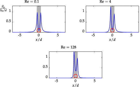
Figure 10. Distribution of  along the x-axis, non-dimensionalyzed with the overall entropy generation rate
  and the diameter d of the bubble.
Download figure:
Standard image High-resolution imageFor spherical bubbles there are asymptotic solutions for Re → 0, associated with the names Hadamard and Rybczinsky, see Clift et al (1978), and for Re → ∞, see Levich (1962). They are


In figure 11 both asymptotes are shown together with our SLA-results (numerical details are given in the appendix). There is a smooth transition between the asymptotic results for small and large Reynolds numbers showing that the integrated entropy generation corresponds to the losses in the flow field for the whole Reynolds number range of laminar flow.
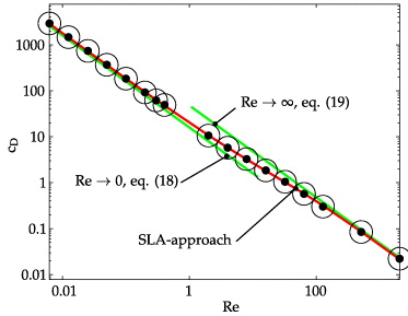
Figure 11. Drag coefficient of a rising spherical bubble numerical results (⊙) and asymptotes shown.
Download figure:
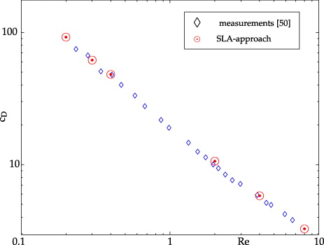
Standard image High-resolution imageA comparison with experimental data in oil, see Peters and Gaertner (2011), as a further validation of the SLA-approach is given in figure 12, here with a close coincidence of experimental and theoretical data.
Figure 12. Drag of small bubbles in oil, measurements from Peters and Gaertner (2011) compared to results with the SLA-approach.
Download figure:
Standard image High-resolution image
5. Conclusions
As an alternative to the conventional definitions of a friction factor for internal flows (based on pressure drop) and a drag coefficient for external flows (based on the drag force) we suggest to uniformly relate them to the entropy generation in the flow field, see table 1.
The advantages of this SLA approach already pointed out in the introduction are
- (i)High accuracy. The integration of entropy generation is performed throughout the entire volume. Thus the presented method is robust against small disturbances which usually appear close to the boundaries of a numerical domain and affect global quantities such as pressure differences or changes in kinetic energies. In addition, it is possible to use a general implementation of the method though the actual cases may differ severely in flow characteristics and geometry.
- (ii)Detailed information about the loss locations. In every example presented here, graphs containing the distribution of losses in streamwise direction have been introduced as an effective visualization method. In these plots both the location of high losses and the influence on the adjacent flow field appear in an easy to understand manner.
- (iii)Physical interpretation in terms of exergy loss. While pressure differences and drag forces do not reveal the actual nature of losses, the SLA directly defines the losses to be losses of available work.
- (iv)Unique assessment when also heat transfer is involved. For cases with heat transfer (not considered in this study) losses in the flow and in the temperature field can uniquely be accounted for by the respective entropy generation. Then the assessment of convective heat transfer situations can be achieved by considering the sum of both as a common quantity instead of comparing friction factors and Nusselt numbers, for example.
Whenever accurate numerical solutions of a flow field in or around certain geometries are available we suggest to at least take into consideration to characterize losses by the alternative way to define friction factors and drag coefficients. Then in a postprocessing step these coefficients can be determined by a volume integral with respect to the local entropy generation rates.
Acknowledgment
The authors gratefully acknowledge the support of the DFG (Deutsche Forschungsgemeinschaft).
Appendix.: Numerical details
All external flow calculations presented in this paper have been performed using OpenFOAM in its version 2.0.0. The flow through the bend was computed using OpenFOAM 1.6. For all cases, a modified version of the standard solver application simpleFoam has been employed to solve the incompressible Navier–Stokes-equations and to compute the  -field within every outer iteration of the coupled solution procedure. The integral value
  thus could be used as a convergence criterion. Calculations were stopped, when the relative change in entropy generation between successive iterations fell below 10−8. The converged solutions on successively refined grids were compared to ensure that a grid independent solution was achieved. Details of the grids and the size of the solution domains are collected in table A.1 for the examples discussed in section 4. Since dimensional quantities were needed for the numerical solution, dummy values for the geometry were employed, which can also be found in table A.1. The kinematic viscosity was chosen such that the velocities in m s−1 have the same value as the Reynolds numbers. Thus, the kinematic viscosities ν in m2 s−1 have the same values as the length scale Lc in m of the corresponding case. The density in μ = ϱν needed for the determination of
  was set to an arbitrary value ϱ = 1 kg m−3. It has, however, no influence on the results since it appears in the numerator as well as the denominator of cD and K, respectively.
Table A.1. Details of the spatial discretization.
| Component | Length of upstream | Downstream-volumes | Diameter/height of num. domain | Char. length | No cells | Simplification |
|---|---|---|---|---|---|---|
| 90° bend | 5Dh | 50Dh | Dh/2 | Dh=2 m | 3 015 000 | Symmetry |
| Flat plate | 10lp | 20lp | 20lp | lp=1 m | 117 600 | 2D, symmetry |
| Bubble/sphere | 17d | 17d | 10d | d=2 m | 139 604 | Axi-symmetry |
| 5° wedge | ||||||
| (azimuthal- | ||||||
| independence) |
A.1. Special aspects for internal flows
For a turbulent internal flow through a bend, developed flow is assumed to prevail at the beginning of the numerical domain. Therefore, profiles for the velocity and the turbulent quantities k and ω for a low Re–k–ω–SST model have to be provided. They are taken from previous simulations of channel flow with periodic boundary conditions for this case, see Schmandt and Herwig (2011b) for details. At the walls, the no-slip boundary condition for the velocity, i.e. ![$\vec {u}=[0,0,0]$](https://content.cld.iop.org/journals/1873-7005/45/5/055507/revision1/fdr481999ieqn57.gif) is applied. Appropriate values for the turbulent quantities are automatically provided by the turbulence model. The level of the so-called kinematic pressure
is applied. Appropriate values for the turbulent quantities are automatically provided by the turbulence model. The level of the so-called kinematic pressure  is set via a fixed value
  adequate for incompressible flow. The pressure at the inlet then is a result of the calculation.
A.2. Special aspects for external flows
Since laminar flow is assumed, the flow situation is given by a far field velocity corresponding to the Reynolds number and the characteristic length scale, only. The velocity ![$\vec u=[u_\infty ,0,0]$](https://content.cld.iop.org/journals/1873-7005/45/5/055507/revision1/fdr481999ieqn60.gif) is given at an upstream cross-section perpendicular to the direction of the main flow. At an opposing downstream cross section the normal gradient of the velocity is set to zero. For the remaining boundary parallel to the direction of the main flow, a slip boundary condition is applied. This boundary condition enforces a parallel flow in the far field. This, however, needs special attention since all components generally lead to a lateral displacement of the massflow. This problem can be circumvented using a numerical domain with a large enough expansion in the direction orthogonal to the direction of the main flow, so that the influence of the body on the far field is small.
is given at an upstream cross-section perpendicular to the direction of the main flow. At an opposing downstream cross section the normal gradient of the velocity is set to zero. For the remaining boundary parallel to the direction of the main flow, a slip boundary condition is applied. This boundary condition enforces a parallel flow in the far field. This, however, needs special attention since all components generally lead to a lateral displacement of the massflow. This problem can be circumvented using a numerical domain with a large enough expansion in the direction orthogonal to the direction of the main flow, so that the influence of the body on the far field is small.
To minimize the grid size, two-dimensional flow and symmetry are assumed for the flat plate while the flow around the sphere and the bubble is assumed to be axi-symmetric. In the latter case, only a wedge with an angle of 5° has to be covered by the grid resulting in a size reduction by a factor 72 compared to a full three-dimensional grid.
A.3. Integration of the entropy generation rates on unstructured grids
The grids used and displayed in the previously described examples from section 4 are generated using the blockMesh utilities from the respective OpenFOAM distributions. This tool is able to generate grids with cells of hexagonal topology. The cells are described via several structured blocks with a prescribed number of divisions in the three spatial directions of each block. Yet, the resulting grid is stored in an unstructured manner.
For various flow situations it is possible to define grids with flat cell layers perpendicular to the direction of the main flow. Among these are the internal flows through smooth pipe bends. With these layers an integration of  at a certain position
  along the path of the main flow can be computed easily. The integral then becomes the scalar product of the
  -field and the scalar field of the single cell volumes, each belonging to cells with cell center coordinates
  . Therefore,
  has to be aligned according to the cell layers. This leads to values
 ![$[\dot S_{\rm D}]_{x=0}^{x=\tilde x} = \dot S_{\rm D} (\tilde x)$](https://content.cld.iop.org/journals/1873-7005/45/5/055507/revision1/fdr481999ieqn66.gif) . A subsequent derivation with respect to x then gives
. A subsequent derivation with respect to x then gives  , see figure 3.
For the flow around the spheres and bubbles, however, it is not possible to generate grids of acceptable quality with cell layers perpendicular to the x-direction. In these cases, some cells are sliced by the clip planes at discrete positions  , now at arbitrary positions not aligned with cell layers. The contribution of the split cells to
  has to be regarded via reduced volumes in addition to the complete cells upstream of
  . Values of
  are always assumed to be constant within each cell. The upstream parts of the divided cell volumes are computed using the convhulln function distributed with Matlab, which is used for the fully automated post-processing. As function input to the convhulln function the grid points of the cut cells located upstream of the clip plane are provided together with the intersecting points of the cell edges with the clip plane. Then the partial volumes appear as an outcome of the convex hull described by these points. Volumes of complete cells, however, are accessed by a customized OpenFOAM utility at much lower computational expense. The whole procedure is enabled by OpenFOAM which stores the grid data as easily accessible compressed ASCII-files. Values, which are not stored in the grid files, like the cell center coordinates, can be computed from the grid data via OpenFOAM utilities and are automatically read by the Matlab post-processing script.