

Abstract
The extensive evaluation studies of the lattice Boltzmann method for micro-scale flows (μ-flow LBM) by the author's group are summarized. For the two-dimensional test cases, force-driven Poiseuille flows, Couette flows, a combined nanochannel flow, and flows in a nanochannel with a square- or triangular cylinder are discussed. The three-dimensional (3D) test cases are nano-mesh flows and a flow between 3D bumpy walls. The reference data for the complex test flow geometries are from the molecular dynamics simulations of the Lennard-Jones fluid by the author's group. The focused flows are mainly in the slip and a part of the transitional flow regimes at Kn < 1. The evaluated schemes of the μ-flow LBMs are the lattice Bhatnagar–Gross–Krook and the multiple-relaxation time LBMs with several boundary conditions and discrete velocity models. The effects of the discrete velocity models, the wall boundary conditions, the near-wall correction models of the molecular mean free path and the regularization process are discussed to confirm the applicability and the limitations of the μ-flow LBMs for complex flow geometries.
Export citation and abstract BibTeX RIS
Communicated by M Funakoshi
1. Introduction
In microfluidics, the representative length H of the flow geometry is sometimes of the order of a few microns. In such a case, since the mean free path λ of gas molecules under atmospheric pressure becomes 0.06 μm, the Knudsen number Kn = λ /H easily reaches Kn > 10- 2 . This condition is known as the slip flow regime where 0.001 <Kn < 0.1 . In the slip flow regime, non-continuum effects are limited to a region adjacent to the wall. This near-wall region known as the Knudsen layer has a larger part of the flow domain at 0.1 <Kn < 10 , which is known as the transitional flow regime. At those finite Kn regimes, the continuum Navier–Stokes equations are no longer applicable and the Boltzmann equation (BE) of the gas kinetic theory is suitable for describing flow physics (e.g. Chapman and Cowling 1970, Cercignani 1975, Karniadakis et al 2005).
Despite the fact that the lattice Boltzmann method (LBM) (e.g. McNamara and Zanetti 1988, Higuera and Jimenez 1989) is a computational method for the Navier–Stokes equations, many attempts to expand the applicability of the LBM for micro-flows such as those in micro/nano-electro-mechanical systems have been made. Those studies on the LBM for micro-flows (μ-flow LBM hereafter) have focused on the slip and transitional flow regimes. Theoretically, the lattice Boltzmann equation (LBE) converges to the Navier–Stokes equations but not to the exact BE due to the discretizations of phase space and time that are tied together (e.g. Saint-Raymond 2009). However, because of its bases, it has been considered that the LBM has potential to be modeled for treating finite Knudsen number flows. Nie et al (2002), Shen et al (2004), Zhang et al (2006a) and Guo et al (2006) showed promising results to describe the finite Kn flows by introducing Kn dependence into the relaxation parameter in the Bhatnagar–Gross–Krook (BGK) model (Bhatnagar et al 1954) of the LBE. Succi (2002) and Sbragaglia and Succi (2005) discussed the specular-reflection and the slip-reflection effects for the wall boundary condition of the slip flow regime, respectively. Toschi and Succi (2005) introduced a virtual wall collision concept into the bounce-back and diffuse-scattering boundary conditions (DSBCs) of Ansumali and Karlin (2002). Zhang et al (2005) applied a Maxwellian scattering kernel to the wall conditions with an accommodation coefficient. Niu et al (2007, 2009) applied the DSBC with the regularization procedure of Zhang et al (2006b) for the non-equilibrium part of the distribution function. (Although a lot more studies on those topics have been published, the relevant reports in the literature are too many to be cited here. A brief summary can be seen in Aidun and Clausen 2010.)
Although most of the μ-flow LBM studies were based on the single relaxation-time lattice BGK (LBGK) model, there have been arguments about the applicability of the LBGK model to the micro-flows. For example, Luo (2004, 2011) argued that the slip velocities predicted by the LBGK model were merely numerical artifacts. (In the Appendix, the discussions on this issue are developed.) Moreover, the LBGK model has viscosity dependence for flow characteristics in complex porous media, whereas the multiple-relaxation-time (MRT) model by d'Humieres et al (2002) does not (Pan et al 2006). Accordingly, Guo et al (2008) discussed the MRT method with the combination of the bounce-back and the specular-reflection wall boundary condition of Succi (2002) for micro-flows. In the context of the MRT LBM, Verhaeghe et al (2009) tested a diffusive bounce-back model for fully diffusive stationary walls. Suga and Ito (2010) then evaluated the μ-flow MRT LBMs by Guo et al (2008) and Verhaeghe et al (2009) in Poiseuille flows and a micro square cylinder flow. They confirmed that although there were still margins to be improved, the MRT model was indeed superior to the LBGK model and the diffusive bounce-back boundary condition was better than the combined bounce-back and specular-reflection boundary condition. Chai et al (2010) considered that a possible way to improve the diffusive bounce-back boundary condition was to connect it with a higher-order slip-flow condition of the modified Reynolds equation of tribology. They thus discussed the second-order slip-flow condition of Hadjiconstantinou (2003) to determine the model coefficients and reported that the Klinkenberg effect (Klinkenberg 1941) was successfully captured. Suga and Ito (2011) further evaluated the MRT model with several slip-flow conditions.
As mentioned above, theoretically the LBE does not converge to the exact BE. With this in mind, when one wants to discuss the applicability of the models in the μ-flow LBMs for engineering simulations, it is readily understood that a model evaluation only in canonical flows is not sufficient. Therefore, the present author's group extensively tested the μ-flow LBMs in micro/nano obstacle flows to confirm their validity by comparing with the data obtained by performing molecular dynamics (MD) simulations (Koplik and Banavar 1995, Haile 1997, etc) of the Lennard-Jones fluid (Suga et al 2010a, 2010b, 2011, Suga and Ito 2010, 2011). According to those studies, this paper summarizes studies to confirm the applicability and the limitations of the μ-flow LBMs in complex flows for practical applications.
2. Mathematical formulation
2.1. Lattice Boltzmann equation by the lattice BGK model
The LBE can be obtained by discretizing the velocity space of the BE into a finite number of discrete velocities ξα { α = 0,1, ... ,Q- 1} . Although many schemes to discretize the velocity space have been proposed, for two-dimensional (2D) and three-dimensional (3D) flows the focused ones in this paper are the so-called 2D nine velocity (D2Q9) and the 3D nineteen velocity (D3Q19) models. (The first part D2 or D3 refers to the dimensionality and the second part Q9 or Q19 refers to the number of discrete velocity vectors.) The velocity models are illustrated in figures 1(a)–(d). Table 1 lists the sound speeds cs , the discrete velocities ξα and the weight parameter ωα in those models. (In table 1, c = δ x/δ t where δ x and δ t are the lattice spacing and the time step, respectively.) Although there are many other versions of the discrete velocity models, when one considers applications to flows in complex geometry, it is readily recognized that multi-level stencils for the discrete velocities such as those used in the D2Q21 and D3Q39 models are not easy to use. They require more than two lattice levels for the streaming, as shown in figures 1(c) and (d). However, in the context of the LBGK model, the D2Q21 and D3Q39 models are also discussed to confirm the effects of those elaborate discrete velocity models in this paper.
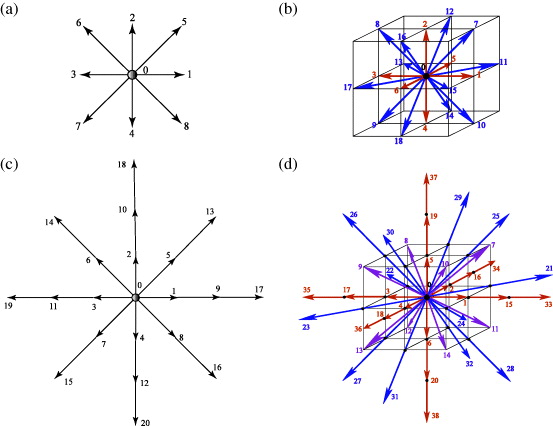
Figure 1. Discrete velocity models: (a) D2Q9 model, (b) D3Q19 model, (c) D2Q21 model and (d) D3Q39 model.
Download figure:
Standard image High-resolution imageTable 1. Parameters of the discrete velocity models for 2D/3D flows.
| Models | cs2 /c2 | ξα /c | ωα |
|---|---|---|---|
| D2Q9 | 1/3 | (0,0) | 4/9(α=0) |
| (±1,0),(0,±1) | 1/9(α=1–4) | ||
| (±1,±1) | 1/36(α=5–8) | ||
| D2Q21 | 2/3 | (0,0) | 91/324(α=0) |
| (±1,0),(0,±1) | 1/12(α=1–4) | ||
| (±1,±1) | 2/27(α=5–8) | ||
| (±2,0),(0,±2) | 7/360(α=9–12) | ||
| (±2,±2) | 1/432(α=13–16) | ||
| (±3,0),(0,±3) | 1/1620(α=17–20) | ||
| D3Q19 | 1/3 | (0,0,0) | 12/36(α=0) |
| (± 1,0 ,0),(0, ± 1 ,0),(0,0, ± 1 ) | 2/36(α=1–6) | ||
| (± 1, ± 1 ,0),( ± 1 ,0, ± 1 ),(0, ± 1, ± 1 ) | 1/36(α=7–18) | ||
| D3Q39 | 2/3 | (0,0,0) | 1/12(α=0) |
| (± 1,0 ,0),(0, ± 1 ,0),(0,0, ± 1 ) | 1/12(α=1–6) | ||
| (± 1, ± 1 , ± 1 ) | 1/27(α=7–14) | ||
| (± 2,0 ,0),(0, ± 2 ,0),(0,0, ± 2 ) | 2/135(α=15–20) | ||
| (± 2 , ± 2 , ± 2 ) | 1/432(α=21–32) | ||
| (± 3,0 ,0),(0, ± 3 ,0),(0,0, ± 3 ) | 1/1620(α=33–38) |
Let x be the Cartesian coordinates of the configuration space and ξ that of the velocity space. The LBE describes evolutions of a single-particle distribution function f(x,ξ ,t) defined such that f(x,ξ ,t) dξ dx represents the number of particles in the phase space element dξ dx at time t , and can be written in the following BGK form (Bhatnagar et al 1954):

where the equilibrium distribution function feq is written as

or

Equation (2) retains up to second-order terms in the Hermite expansion and used in the D2Q9/D3Q19 model whereas equation (3) retains further up to third-order terms and used in the D2Q21/D3Q39 model. The ideal gas constant is R and ρ , u and T are, respectively, the fluid macro density, velocity and temperature. The sound speed is  and varies by the discrete velocity models as shown in table 1. (As already described in many review papers such as the one by Chen and Doolen (1998), it is well understood that such an unphysical relation needs compromising in the iso-thermal LBM systems.) The contribution of the force Fα is introduced respectively for the D2Q9/D3Q19 and D2Q21/D3Q39 models as

where a is the acceleration vector of the force and the second-order Hermite polynomial is H(2) (ξα ) = ξα i ξα j - δij.
The variables ρ , u, pressure p , viscosity μ and stress tensor σ are respectively obtained by
2.2. MRT lattice Boltzmann equation
The MRT LBM (d'Humieres et al 2002) transforms the distribution function in the velocity space to the moment space by the transformation matrix M. Since the moments of the distribution function correspond directly to flow quantities, the moment representation allows us to perform the relaxation processes with different relaxation times according to different time scales of various physical processes. The evolution equation is thus written as
where the notation such as  is
is  , I is the identity matrix and δ t is the time step. The term F is an external body force:

where ρ0 is the mean density of the system that is set to be unity.
The matrix M is a Q × Q matrix that linearly transforms the distribution function to the moment:  . For the D2Q9 model, the transformation matrix is
Its collision matrix  is diagonal:

The moment components have physical significance:

where the density ρ and the momentum j = ρ u = (jx ,jy ) are conserved moments. The other six non-conserved moments, e , ε , q = (qx ,qy ) , pxx and pxy , are, respectively, related to energy, energy square, energy flux, and diagonal and off-diagonal components of the stress tensor. The equilibria of the conserved moments are themselves and those of the non-conserved moments are products of the conserved moments:


For the D3Q19 model, the transformation matrix is
and the components of the corresponding moment are

where mi and πii are the cubic- and fourth-order polynomials of the momentum, respectively. Note that pww = pyy - pzz and πww = πyy - πzz . The equilibria of the moments are functions of the conserved moments and given as


To recover the corresponding LBGK model, the parameters need to be ωε = 3 , ωxx = - 1/2 , ωε j = - 11/2 . However, d'Humieres et al (2002) recommended their optimized parameters: ωε = 0 , ωxx = 0 , ωε j = - 475/63 through the linear analysis for stability of Lallemand and Luo (2000).
The collision matrix is written as

for the D2Q9 model, and for the D3Q19 model, it is

where the subscript of the relaxation rates corresponds to the physical significance. The kinetic viscosity ν = μ /ρ and the bulk viscosity ζ are given as


2.3. Kinetic boundary conditions
Since the conventional bounce-back boundary condition does not apply to the slip-flow boundary condition, several boundary conditions have been proposed for micro-flow simulations. In this paper, some of the representative ones are applied. They are the diffuse-scattering, bounce-back specular-reflection and diffusive bounce-back wall boundary conditions.
2.3.1. Diffuse-scattering boundary condition (DSBC).
The non-slip wall boundary conditions used in the continuum LBM are based on perfect reflection, so the velocity and the temperature of a wall are not reflected in the distribution of the reflected particles. However, from a microscopic viewpoint, the wall boundary condition should include the physics on the wall because the fluid and the wall molecules interact with each other. Therefore, the incident particles are modeled to reflect the information of the Maxwell distribution function at the wall boundary. The modeled form (Ansumali and Karlin 2002) is written in the LBM frame as
where n is the unit wall normal vector, ξ 'α is the velocity of incident particles, fα ,weq is the wall equilibrium distribution function, and the subscripts w,α ',α respectively denote the wall and the directions of the incident and reflected particles.
2.3.2. Bounce-back specular-reflection boundary condition (BSBC).
Succi (2002) proposed the combined bounce-back and specular-reflection boundary condition for slippage at a solid wall in a micro-flow. In this scheme, it is assumed that some of the particles hitting the solid wall bounce back but the others reflect specularly. It is expressed as

where rs is a bridge coefficient taking rs = 0.0 - 1.0 and vectors ξβ = - ξα and ξγ = ξα - 2(ξα ⋅ n)n are, respectively, the inverse and the specular symmetric velocity vectors of ξα .
In the context of the MRT model, by discussing the second-order slip boundary condition for the microscopic slip velocity, Guo et al (2008) derived the bridge coefficient as

where τs = 1/sν,  , τs (0) = τs |wall , τ 's (0) = ∂ τs /∂n|wall and n is the wall-normal direction. The coefficients are
  ,
,  and σa is the accommodation coefficient.
2.3.3. Diffusive bounce-back wall boundary condition (DBBC).
The diffusive bounce-back boundary condition is the combination of the above diffuse-scattering and bounce-back boundary conditions for the wall boundary as

where r is a probability coefficient taking r = 0.0 - 1.0 , the bounce-back vectors are ξβ = - ξα and fα D is the diffuse scattering model given by equation (20). This model turns into the diffuse scattering model when r = 1 , while it becomes the (non-slip) bounce-back model with r = 0 .
In the context of the MRT LBM with the D2Q9 model, the DBBC describes the velocity at near-wall lattice node 2 as

where Uj is the velocity at lattice node j and ax is the acceleration parallel to the wall (i.e. a = (ax ,0) ). When lattice nodes 1 and 2 are located at δ x/2 and 3δ x/2 from the wall (the wall is situated halfway between nodes 0 and 1 as shown in figure 2), Chai et al (2010) obtained the parameters A1 and A2 as

where τν = sν - 1 and τq = sq- 1 . In a fully developed 2D Poiseuille flow in the slip flow regime, by integrating the momentum equation with the second-order boundary condition,

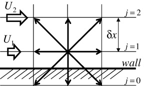
Figure 2. Near-wall configuration of the D2Q9 model.
Download figure:
Standard image High-resolution imageFor coefficients C1 and C2 , there are many proposals by the kinetic theory (e.g. Mitsuya 1993, Beskok et al 1996, Hadjiconstantinou 2003). When the velocity distribution is assumed to be parabolic, the velocity can be described as

where H is the channel height and Uc is the centerline velocity: Uc = ax H2 /(8ν ) . Thus, the slip velocity at the wall can be obtained as

By equations (24), (25) and (27), one can obtain
Comparing equations (28) and (29), one can derive

as in Chai et al (2010).
Verhaeghe et al (2009) applied only the first-order terms of equations (28) and (29) and their expression for r was

where c = δx/δt. (Equation (30) can be rewritten as equation (32) when c = C1.) With this first-order slip velocity condition, Verhaeghe et al (2009) applied

following Ginzbourg and Adler (1994). When r = 0 for the pure bounce-back boundary condition, it is recognized that this condition of equation (33) guarantees Us = 0 by equation (29).
2.4. Correction of the molecular mean free path
In microscale wall bounded geometries, the mean free path of the total molecules in the system should be smaller than that in the unbounded systems due to the wall effects. Stops (1970) then introduced a correction function Ψ (Kn) to the molecular mean free path as

According to the gas kinetic theory, the molecular mean free path can be related to the dynamic viscosity,  (Succi 2002), and thus the relaxation time τ can be expressed as
  . The effective relaxation time τ
* can be modeled as
. The effective relaxation time τ
* can be modeled as

where Kn in λ
* (equation (34)) is the representative Knudsen number without considering the local effects:  , where subscript 0 means the reference value in the flow system considered. However, as in the studies by Suga et al (2010a, 2010b), it can be defined using the local density to include local effects as

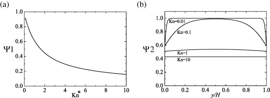
The function Ψ derived by Stops was very complicated and difficult for practical applications. Guo et al (2006) thus approximated the function by a simple formula as

This correction model is referred to as the Ψ 1 model in the following discussions. As shown in figure 3(a), the functional behavior (Ψ decreases as Kn* increases) indicates that some molecules will hit walls and their flight time may be shorter than the mean free time (relaxation time τ ) defined in an unbounded system.
Download figure:
Standard image High-resolution imageZhang et al (2006a) used a wall function to simulate the Knudsen layer. Their wall function is a function of the wall normal distance y. The form is

where the chosen coefficient is C = 1 . In Poiseuille and Couette flows, the form

was applied. This model is referred to as the Ψ 2 model in the following discussions. Its functional behavior is plotted in figure 3(b). Zhang et al (2006a) claimed that this model captured the Knudsen layer with reasonable description of the nonlinear flow characteristics up to Kn ≈ O(1) .
In the context of the MRT LBM, the mean free path is expressed as

by the gas kinetic theory and thus equation (18) can be rewritten as

since p = ρ RT = ρ cs2 .
2.5. Regularization procedure
Generally speaking, the computed distribution function f includes an error because it cannot be entirely projected onto the Hermite space. Such an error is usually very small, but it can be no longer neglected when the system is far from equilibrium because of finite Knudsen number effects. Therefore, to resolve this problem by canceling unnecessary higher-order contributions to the non-equilibrium distribution functions for guaranteeing the non-equilibrium moments of the LBE to satisfy the Hermite space, Latt and Chopard (2006) and Zhang et al (2006b) introduced the regularization procedure. The procedure is implemented before the collision step as the following. Firstly, the distribution function f is divided as

where f' is the non-equilibrium part of the distribution. Secondly, it is necessary to convert f' to a new distribution  that lies within the subspace spanned by the higher-order Hermite polynomials. The non-equilibrium distribution function f' (=f'α ) is projected on the Nth order of the truncated Hermite expansion:
 ![$\skew3\tilde f'_{{\alpha}} = \omega _{{\alpha}} \sum\nolimits_{n = 0}^N {\left[ {\frac{1}{{n!}}C^{(n)} {\bf{H}}^{(n)} ({\boldsymbol{\xi }}_{{\alpha}} /c_{\rm s} )} \right]} ,$](https://content.cld.iop.org/journals/1873-7005/45/3/034501/revision1/fdr470526ieqn13.gif) with the Hermite expansion coefficients
with the Hermite expansion coefficients  . For the D2Q9/D3Q19 and D2Q21/D3Q19 models,
  is written in the generic form by using mass and momentum conservation as

where the coefficient B is given as B = 1 - Ψ and H(3) (ξα ) = ξα i
ξα j
ξα k - ξα i
δjk - ξα j
δik - ξα k
δij is the third-order Hermite polynomial of ξα . By the expression of equation (42) replacing f'α with  of equation (43) or (44), one can rewrite equation (1) as

For the MRT model, the corresponding form is
The distribution function f is thus expressed by the second- or third-order truncated Hermite expansions. It means that the higher-order terms in the non-equilibrium distribution, which are from numerical errors and even physical processes, are filtered out and the regularization enforces the system to be confined within the second- or third-order Hermite moment space, respectively, for the D2Q9/D3Q19 and D2Q21/D3Q19 models.
3. Results and discussions
All the simulation results presented here were obtained by the in-house LBM code 'POLAS 2D/3D (Parallelized Orthogonal Lattice–Boltzmann Automata Solver 2D/3D)' developed by the author's group (Suga and Nishio 2009). The reference data of complex flows were obtained by performing MD simulations of the Lennard-Jones fluid by the author's group. (For details, see Suga et al
2010a, 2010b, 2011, Suga and Ito 2010, 2011.) In the LBM simulations, the reference Knudsen numbers are explicitly given to determine the relaxation time as  .
.
3.1. Fundamental aspects
3.1.1. Slippage velocity and flow rate.
Niu et al (2007) and Suga et al (2010b) confirmed that the D2Q21 LBGK LBM with the DSBC reasonably captured Knudsen number effects in channel flows. This can be confirmed in figure 4 where the velocity profiles of plane Poiseuille channel flows at Kn = 0.01–10 are compared with the data of the DSMC (Beskok and Karniadakis 1999). (Figures are re-plotted for this paper with re-calculated data.) These velocity profiles are normalized by the bulk mean velocity Ub . The 2D uniform Cartesian lattice whose wall normal node points are 100 (this density of the lattice was confirmed to be more than good enough) is used for the simulations. The correction function of the molecular mean free path Ψ 1 and the regularization procedure are coupled with the LBGK LBM. It can be seen that the less accurate discrete velocity model of the D2Q9 model also captures the increasing level of the slip velocity due to Kn and velocity profiles, although its results always deviate a little from those of the DSMC very near the walls, particularly when Kn ⩾ 0.1 . This is partly because in the D2Q9 model, only up to second-order terms are retained in the Hermite expansion of the Maxwellian distribution while the D2Q21 model retains terms of third-order in the Hermite expansion and uses a Gauss–Hermite quadrature of third-order to obtain the discrete velocity values. Note that the D2Q21 and D3Q39 models require three levels of particle velocity. For particles with two and three unit speeds, when the DSBC is applied, it is necessary to provide information of nodes inside the wall (pseudo nodes). In such cases, the wall surface values are simply taken for those pseudo nodes.
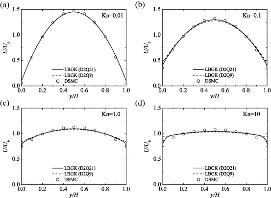
Figure 4. Velocity profiles by the LBGK LBM in Poiseuille flows: (a) at Kn = 0.01, (b) at Kn = 0.1, (c) at Kn = 1.0 and (d) at Kn = 10; all the results are by coupling with the DSBC, the regularization and Ψ 1 ; the DSMC data are from Beskok and Karniadakis (1999).
Download figure:
Standard image High-resolution imageFigure 5 compares the dependence of the flow characteristics on Kn. Figure 5(a) compares the slippage and centerline velocities: Us and Uc . The D2Q21 model shows better agreement with the reference data (Karniadakis et al 2005). As shown in figure 5(b), as for the distribution of the normalized mass flow rate,

where ax is the streamwise acceleration, both the D2Q21 and D2Q9 models predict reasonable results at least when Kn < 1. (Some comments on the slippage velocity by the LBGK LBM are in the Appendix.)
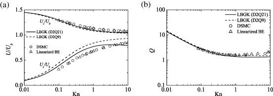
Figure 5. Dependence of the flow characteristics on Kn by the LBGK LBM: (a) velocity scaling at wall and centerline of the channels and (b) flow rates; all the results are by coupling with the DSBC, the regularization and Ψ 1 ; the reference data are from Karniadakis et al (2005).
Download figure:
Standard image High-resolution imageIn order to know the performance of the MRT LBMs with the DBBC to predict slippage velocities and flow rates, the same flow fields were discussed by Suga and Ito (2011). The compared LBMs were the MRT LBMs with the D2Q9 by the first-order and second-order slip-flow models. The first-order slip-flow model was the one proposed by Verhaeghe et al (2009) whereas one of the second-order models was Hadjiconstantinou's (2003) model, which applies C1 = 1.11, C2 = 0.61 , following the recommendation by Chai et al (2010). Another second-order model was Mitsuya's model, which was denoted the 1.5th-order model following the original naming by Mitsuya (1993). It applies C1 = 1.0, C2 = 2/9 . These coefficients are summarized in table 2.
Table 2. Coefficients of the slip-flow models.
| Slip-flow model | C1 | C2 |
|---|---|---|
| First order | 1.0 | – |
| 1.5th order | 1.0 | 2/9 |
| Second order | 1.11 | 0.61 |
Figure 6(a) compares the slip and centerline velocities: Us and Uc . Although each agreement is not good enough at Kn > 0.1 (Us is overpredicted up to 20% of Ub and Uc is underpredicted up to 10% of Ub ), the profiles of Us and Uc by each model correspond well with the reference data at Kn ≈ 0.1. However, as shown in figure 6(b), for the mass flow rate the 1.5th-order slip-flow model leads to the best agreement among the slip-flow models. Interestingly, each profile shown in figure 6(b) corresponds well to the analytically obtained distributions in Mitsuya (1993). Only the different points in the model terms are the values of the probability coefficient r and the relaxation time τq for the energy flux. By equation (30), the probability coefficient is fixed as r = 0.84,0.84 and 0.89 by the first-order, 1.5-order and second-order slip-flow models, respectively. The relaxation time τq varies a lot depending on the Knudsen number. At Kn = 0.01, τq = 0.64,0.88 and 1.29 while it is 0.50, 239.26 and 655.96 at Kn = 10 by the first-order, 1.5-order and second-order slip-flow models, respectively, when the channel height is divided into 99 lattice spaces. Consequently, at Kn ≪ 0.1 , the difference in the values of r or τq is not significantly large and this results in nearly the same results of the flow characteristics. However, at Kn ≫ 1 , the difference in the values of τq becomes very large and accordingly it affects the predicted behavior such as the flow rate shown in figure 6(b).
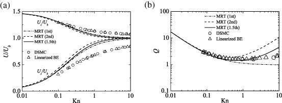
Figure 6. Dependence of the flow characteristics on Kn by the MRT LBM with the first-, 1.5th- and second-order slip flow DBBCs: (a) velocity scaling at wall and centerline of the channels and (b) flow rate. Figures taken from Suga and Ito (2011). Copyright 2011, Tech Science Press.
Download figure:
Standard image High-resolution imageIt is recognized that the regularization procedure filters the majority of such differences out. As shown in figures 7(a) and (b), with the regularization procedure, all the slip-flow models produce nearly the same flow characteristics even at Kn > 1. This means that with the regularization, the order of the slip-flow model may not be very important. A similar effect to that shown in figures 6(b) and 7(b) was reported by Zhang et al (2006b) for the same force-driven Poiseuille flows. They discussed the effect of the regularization on the flow rate tendency by the D2Q9 BGK model with the bounce-back boundary condition and found that by the regularization process, only the Navier–Stokes order effects were preserved in their result (which was much worse than in figure 7(b)). Their conclusion was that since the regularization enforced the system to be confined within the second-order Hermite moment space in the D2Q9, all the higher-order non-equilibrium contributions from both the numerical and physical processes responsible for the finite Knudsen phenomena were filtered out. Although their sub-models for the micro-flows such as for the relaxation time and the boundary condition are different from the results shown in figure 7, due to the similar mechanisms, it is considered that the difference in the slip-flow models is reduced. The effects of the regularization become more obvious in the complex flow geometry discussed later.
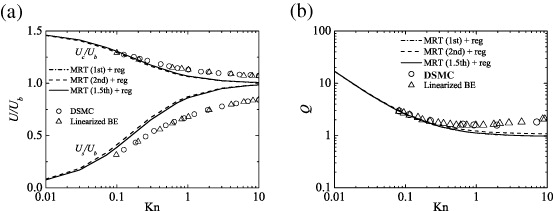
Figure 7. Effects of the regularization on the flow characteristics by the MRT LBM with the first-, 1.5th- and second-order slip flow DBBCs: (a) slip and centerline velocities and (b) flow rates. Figures taken from Suga and Ito (2011). Copyright 2011, Tech Science Press.
Download figure:
Standard image High-resolution image3.1.2. Knudsen layer effects.
Since the LBE does not converge to the BE, it is difficult to capture the Knudsen layer effects precisely. However, due to the models incorporated, it has often been reported that the LBM can capture them. Therefore, in this part of the section, the model performance is evaluated by the numerical solutions.
The near-wall velocities particularly with the correction Ψ of the mean free path are expected to show different profiles from the parabolic ones since Ψ was designed to take into account the characteristic Knudsen-layer effects. In order to investigate the Knudsen-layer correction by Sone (2007), analyses using the Couette flow simulations are performed as in Suga et al (2010b). In the Couette flows at a constant temperature, the Knudsen-layer correction of Sone reduces to

where
UGw - Uw is the virtual slip velocity which is the difference between the wall velocity Uw and the velocity UG at the wall. As illustrated in figure 8(a), UG is the velocity extrapolated from the Navier–Stokes velocity profile in the bulk region. The Knudsen-layer correction of the velocity UK is the difference between the velocity in the Knudsen layer and UG : UK = U- UG . As shown in figure 8(b), both correction models Ψ 1 (equation (37)) and Ψ 2 (equation (39)) seem to reproduce well the solution of Sone (2007). Here the first-order slip flow DBBC and the regularization are applied to the MRT LBM by the D2Q9. However, Ψ 1 and Ψ 2 models predict the slip coefficient as k0 = - 1.0664 and - 1.1705 at Kn = 0.11 while it is k0 = - 1.01619 for the BGK model irrespective of Kn by Sone (2007). Moreover, as shown in figure 8(c), the predicted profiles of the Knudsen-layer function Y0 (ηKL ) are too large or one order smaller than that obtained by Sone. Here, ηKL is the Knudsen-layer coordinate defined as  . (The profile of Ψ 1 by the D2Q9 model is almost invisible at the scale used.) In figure 8(c), the results by the LBGK LBMs with the DSBC are also compared. Generally, all the shown tendencies by Ψ 2 are the same and it is confirmed that the results are insensitive to the discrete velocity models except in the vicinity of the wall. Although the profiles are not shown here, at Kn = 1.1 even with the D2Q21, both the correction models predict the profiles that are not visible with the same scale of figure 8(c). These results are consistent with the discussions by Watari (2010), who proved that to reproduce the relaxation process in the Knudsen layer, the triple octagon model with 24 velocity directions, which was too elaborate to apply for complex geometry, was required.
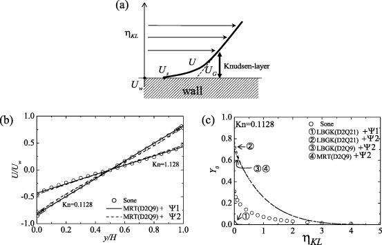
Figure 8. Comparison of the velocity profiles of Couette flows and the Knudsen-layer function: (a) schematic view of the Knudsen layer, (b) comparison with the velocity profiles of the Couette flows by Sone (2007) and (c) profiles of the Knudsen-layer function; the DSBC is applied to the LBGK while the first-order slip flow DBBC is applied to the MRT; the regularization is applied to all the models.
Download figure:
Standard image High-resolution imageTherefore, it is confirmed that even though some correction model or wall function seems to work well to predict the Knudsen layer effects, we cannot generally expect much for the accuracy of the prediction of the Knudsen layer. This is consistent with the comments by Luo (2011). However, the correction of the mean free path is useful particularly for predictions of the slip velocity at Kn > 0.1 as shown in figure 9(a) whereas the flow rates are rather insensitive as in figure 9(b).
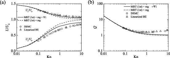
Figure 9. Effects of the correction of the mean free path in Poiseuille flows: (a) slip and centerline velocities and (b) flow rates; the first-order slip flow DBBC and the regularization are applied to all the models.
Download figure:
Standard image High-resolution image3.2. Complex flows in the slip-flow regime
In order to discuss further the applicability and limitations of the μ-flow LBM, 2D and 3D complex flow geometries were discussed (Suga et al 2010a, 2010b, 2011, Suga and Ito 2010, 2011). Since there were not enough bench-mark test data of complex micro-flows in the literature, by performing MD simulations (Koplik and Banavar 1995, Haile 1997, etc) of the Lennard-Jones fluid, they obtained the reference data in the slip-flow regime at Kn ≈ 0.1 . Note that even for obtaining 2D flow statistics, a 3D flow field should be considered in the MD simulation. To compare the results of the LBM with those of the MD simulations, we need to normalize the flow profiles since only Kn is the common number between them and it is also necessary to eliminate the dependence of local flow conditions. For normalization of the velocity profiles, maximum velocity, inlet velocity, etc can be the candidates of the reference value to compare the velocity profiles.
3.2.1. Effects of the regularization.
Suga et al (2010b) discussed the flows in a nanochannel with a square cylinder placed at the center region, which is shown in figure 10 and called square cylinder flow hereafter. Periodic boundary conditions were applied to each direction and thus the flow regime was regarded as a part of an infinite cylinder array set in a nanochannel. The force was applied to the x-direction only and the simulations were carried out on the 2D grid whose size was 100 × 100 , which was confirmed to be good enough for grid-independent solutions.
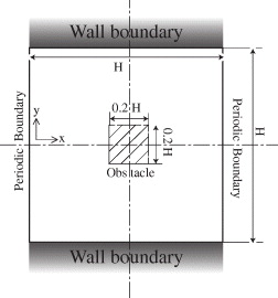
Figure 10. Schematic view of the flow field geometry of the flow around a square cylinder in a nanochannel. Figure taken from Suga et al (2010b). Copyright 2010, American Physical Society.
Download figure:
Standard image High-resolution imageFigure 11 shows contour maps of the streamwise velocity magnitude calculated by the LBGK LBM with the DSBC. As is clearly seen, without the regularization procedure, the predicted flow field shows unphysical patterns around the cylinder (figure 11(b)). Although this tendency was not so strong, it was also confirmed in the lower Kn cases. When the projection of the LBE into the Hermite space is considered, it is understood that the collision step introduces an error because the distribution function does not automatically lie entirely within the Hermite space. In the case that the system is not far from equilibrium, such an error is small and can be ignored (Zhang et al 2006b). Latt and Chopard (2006) argued that since the number of distribution functions was normally greater than that of flow variables, the set of unknowns could be considered as overdetermined and thus the non-equilibrium part of the distribution included higher-order moments in principle. It is considered that this contribution of the non-equilibrium part of the distribution tends to be greater as Kn increases. However, the regularization procedure filters such higher-order non-equilibrium moments out, and the resultant flow field becomes dealiased. It can thus be considered that even though LBMs without the regularization work reasonably well at moderate Kn in wall parallel flows (the majority of the LBMs in the literature are in this category), their performance in complex micro-/nano-flows may be questionable.
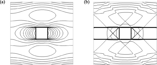
Figure 11. Contour maps of streamwise velocity magnitude at Kn = 1.0: (a) with regularization and (b) without regularization; all the results are by coupling with Ψ 1 . Figures taken from Suga et al (2010b). Copyright 2010, American Physical Society.
Download figure:
Standard image High-resolution image3.2.2. Effects of discrete velocity models.
Figure 12 compares the normalized streamwise velocity U profiles by the LBGK model with the DSBC, the regularization and Ψ 1 at x/H = 0.0, 0.25, 0.5, 0.75 for the case of Kn = 0.11. The distribution profiles of the D2Q9 and D2Q21 models agree well with those of the MD simulation. Since it can be seen that the profiles of the D2Q9 model are also acceptable and the maximum difference from those of the D2Q21 model is less than 5% of the bulk mean velocity, the conventional D2Q9 model can also be applicable to simulate the velocity profiles of the complex micro-flow. Although Suga and Ito (2011) confirmed that slightly more satisfactory results were obtained by the MRT LBM with the D2Q9 model as shown in figure 13, the results of the LBGK models in figure 12 are also acceptable. Note that it is clear in figure 13 that with the regularization, the slip-flow models applied to the DBBC do not provide any difference as in the Poiseuille flows.
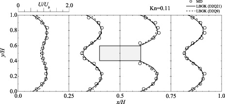
Figure 12. Comparison of streamwise velocity profiles by the LBGK LBM in the square cylinder flow at Kn = 0.11; all the results are by coupling with the DSBC, the regularization and Ψ 1 .
Download figure:
Standard image High-resolution image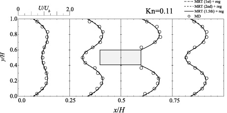
Figure 13. Comparison of streamwise velocity profiles in the square cylinder flow by the MRT LBM with the first-, 1.5th- and second-order slip flow DBBCs, the regularization and Ψ 1 at Kn = 0.11. Figure taken from Suga and Ito (2011). Copyright 2011, Tech Science Press.
Download figure:
Standard image High-resolution image3.2.3. Effects of wall BCs.
For discussing the flow characteristics by the wall boundary conditions in a developing nano-flow, flow in a nanochannel with an inserted flat plate was considered in Suga et al (2010a). As shown in figure 14, the mother channel with height H and domain length L had an inserted flat plate, which made another narrower channel region. The thickness and the length of the plate were 0.15H and L/2, respectively. The gap (the height of the finite narrower channel) between the plate and the channel bottom wall was 0.125H. The drive force and periodic boundary conditions were applied to the x-direction, and thus the flow regime was regarded as a fully developed force-driven nanochannel flow combined with developing narrower nanochannel flows inside. The considered Knudsen number was Kn = 0.14 based on the characteristic length H. The LBGK LBM simulations were carried out on a grid of 187 × 97 , which was confirmed to be good enough.
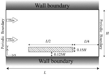
Figure 14. Flow field geometry of the combined nanochannel. Figure taken from Suga et al (2010a). Copyright 2010, Global Science Press.
Download figure:
Standard image High-resolution imageFigure 15 compares the normalized streamwise velocity U profiles at x/L = 0.0 - 0.76 . Both the LBGK simulations were coupled with the regularization and Ψ 1 . The results with the DSBC agree with the profiles of the MD simulation with an error of up to 10% of Ub in the wider gap region. Although the slip and centerline velocities of Poiseuille flows were confirmed to be satisfactorily predicted by the BSBC model with b = 0.7 at Kn ⩽ 0.14 , the BSBC model produces less slippage velocities and greater centerline velocities (with up to 20% of Ub ) in figure 15. The initial flow development in the narrower channel at x/L = 0.22 does not satisfactorily agree with the MD profile although the DSBC provides better results. Hence, it can be recognized that the bridging coefficient for the BSBC model needs some dependence on local flow quantities.
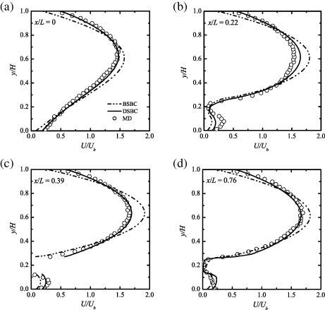
Figure 15. Comparison of the effects of the boundary conditions in the development of streamwise velocity profiles of the combined nanochannel flow by the LBGK LBM coupled with the regularization and Ψ 1 at Kn = 0.14. Figures taken from Suga et al (2010a). Copyright 2010, Global Science Press.
Download figure:
Standard image High-resolution image3.2.4. Applicability to complex shapes: Interpolated BC.
To discuss further the applicability to the complex flow geometry, as shown in figure 16, Suga and Ito (2011) considered a force-driven flow in a nanochannel with a triangular cylinder at the center region, which is called triangular cylinder flow hereafter. To describe the slanted faces of the triangular cylinder, an interpolation scheme was applied since Peng and Luo (2008) concluded that the accuracy of the interpolated bounce-back (IBB) boundary condition was better than that of the immersed-boundary method. Although they chose the quadratic IBB, there was no significant difference between the quadratic and linear IBB in Pan et al (2006). Thus, the linear IBB was applied.
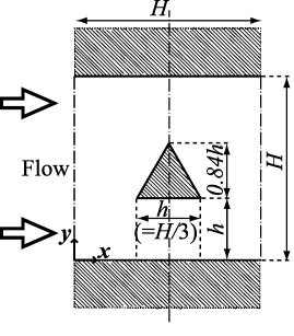
Figure 16. Schematic view of the flow field geometry of the flow around a triangular cylinder in a nanochannel. Figure taken from Suga and Ito (2011). Copyright 2011, Tech Science Press.
Download figure:
Standard image High-resolution imageFigures 17(a)–(c) illustrate the procedures of the linear IBB boundary condition of Pan et al (2006) in a one-dimensional setting. As shown in figure 17(a), when the boundary xW is located at the middle between nodes xA and xB (q = |xA - xW |/|xA - xB | = 1/2 ), the particle at node xA travels and collides with the wall at xW and reverses its momentum (the collision process completes instantly), then travels back to xA . Thus, the incoming distribution function is simply equal to the corresponding outgoing one with the opposite momentum. This is the so-called halfway bounce-back (HWBB) condition and accurate in this case. The IBB condition thus generalizes the HWBB condition. When q < 1/2 as in figure 17(b), the particle at xA should end up at xC after the streaming–collision cycle. Likewise, the particle starting from xC ends up at xA after the streaming–collision cycle. This is accomplished by interpolating the distribution function for xC before the streaming–collision process with the wall takes place. Similarly, when q > 1/2 as in figure 17(c), the incoming distribution function can be obtained by using the outgoing one located at xC after the streaming–collision interaction with the wall takes place and the distribution function values at nearby nodes xD and xE . Thus, the linear IBB formulae for  may be written as
where f and  respectively denote the post- and pre-collision states of the distribution function. The subscripts L and R indicate left- and right-bound directions, respectively.
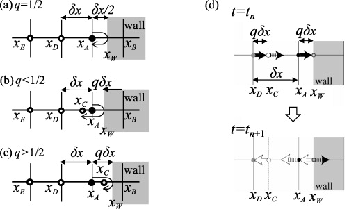
Figure 17. IBB and diffuse scattering boundary conditions: (a)–(c) linear IBB scheme and (d) linear IDS scheme. Figures taken from Suga and Ito (2011). Copyright 2011, Tech Science Press.
Download figure:
Standard image High-resolution imageIn order to represent the curved surfaces, an interpolation scheme is also applied to the diffuse scattering boundary condition, which is called the interpolated diffuse scattering (IDS) boundary condition. As schematically shown in figure 17(d), the distribution functions can be interpolated as


The D2Q9 MRT LBM simulations with the IDBBC, the regularization and Ψ 1 were carried out on the 2D grids at the corresponding Kn = 0.14 to that of the MD result. The applied computational grid was 96 × 96 . Figure 18 compares the velocity profiles in the triangular-cylinder flow. As clearly seen in figure 18(a), without the regularization procedure, the distributions along the slant face at x/H = 0.43 and 0.5 are very different and show unphysical shapes, particularly by the 1.5th- and second-order slip-flow models. Indeed, with the higher-order slip-flow model, the slip velocity at the peak of the triangle tends to be oscillating as noticed in the profiles at x/H = 0.5 . As discussed before, such oscillations can be dealiased by introducing the regularization procedure. With the regularization process, the oscillations and discontinuity in the profiles disappear, as shown in figure 18(b). (As discussed so far, all the slip-flow models produce virtually the same velocity profiles as in figures 18(b) and (c).) It can also be observed that the discrepancy between the MRT LBM and the MD results is up to 20% of Ub at the most difficult position to predict.
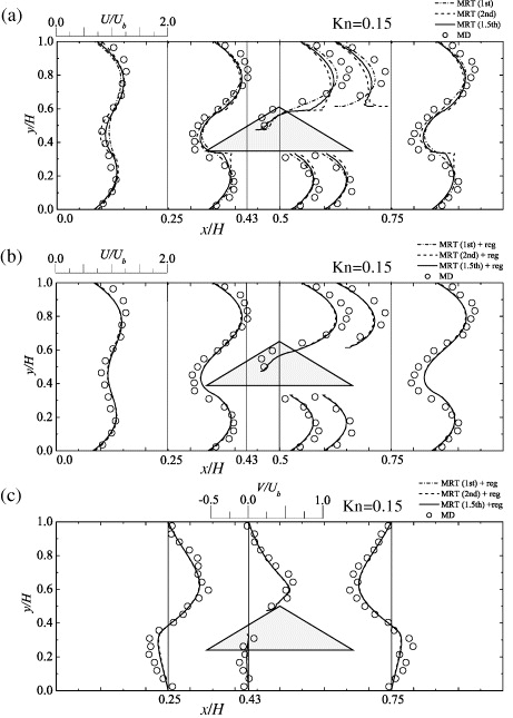
Figure 18. Comparison of velocity profiles around a triangular cylinder in a nanochannel by the MRT LBM with the first-, 1.5th- and second-order slip flow IDBBCs, the regularization and Ψ 1 at Kn = 0.15: (a) streamwise velocity component profiles without the regularization process, (b) streamwise velocity component with the regularization process and (c) vertical velocity component with the regularization process. Figures taken from Suga and Ito (2011). Copyright 2011, Tech Science Press.
Download figure:
Standard image High-resolution image3.2.5. Effects of the 3D discrete velocity models.
To confirm the tendencies observed in the 2D flows, 3D nano-mesh flows were discussed. Figure 19 illustrates a schematic view of the nano-mesh flow of Suga et al (2011). Since the periodic boundary condition was applied to each direction, this flow domain represented a kind of mesh geometry whose porosity was φ = 0.88 . This geometrical structure of the nano-mesh is similar to that of a model structure of cellular foams (e.g. Du Plessis and Masliyah 1988, Fourie and Du Plessis 2002). The force corresponding to a mean pressure gradient was applied to the x-direction. The characteristic Knudsen numbers from the MD simulation results were Kn = λ /dh = 0.1 and 0.2 where dh was the mean hydraulic diameter of the nano-mesh: dh = 0.43H. The LBGK LBM simulations with the DSBC, the regularization and Ψ 1 were carried out on a regular uniform grid of 100 × 100 × 100 at the corresponding Kn. (After a series of grid dependency tests using grids of 40 × 40 × 40 , 100 × 100 × 100 and 140 × 140 × 140 , the results by the grid of 100 × 100 × 100 were confirmed to be enough for grid-independent solutions.)
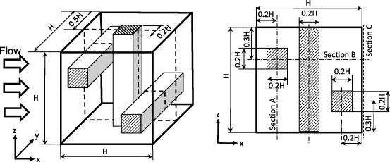
Figure 19. Schematic view of the computational domain for the nano-mesh; periodic boundary conditions are applied to all the boundary faces. Figure taken from Suga et al (2011). Copyright 2011, Inderscience Enterprises.
Download figure:
Standard image High-resolution imageFigures 20(a)–(f) respectively compare the distribution profiles of the velocity U in the x -direction at sections A, B and C indicated in figure 19 at Kn = 0.1 and 0.2. (The figures are re-plotted with the additional data of the MRT LBM with the first-order slip-flow DBBC for this paper.) All the sections are in the symmetry plane of y/H = 0.5 as in figure 19. It is clearly shown that both the results of the LBGK simulations by the D3Q19 and the D3Q39 models agree with those of the MD simulation. Most of the LBM results are in the fluctuation range of the MD results although the LBM simulations predict peak velocities lower than those by the MD simulation at z/H = 0 and 1.0 in figures 20(a), (e) and (f). The discrepancies of the results are up to 20–30% of Ub . These discrepancies come from the predicted slip velocities at the wall surfaces. Since the LBM predicts slightly larger slip velocities at some locations as shown in figure 20(c) for example, the corresponding peak velocity distribution tends to be lower. It is also clear that the difference between the two discrete velocity models is small. It can also be seen that the difference between the results of the LBGK LBMs and the D3Q19 MRT LBM with the DBBC is marginal. Indeed, the results of the D3Q19 MRT LBM almost perfectly overlap with those of the D3Q39 LBGK LBM.
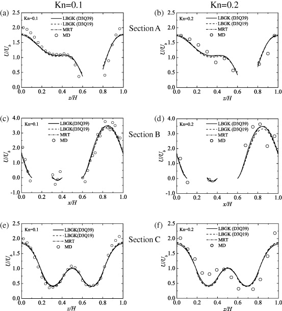
Figure 20. Comparison of velocity profiles in the nano-mesh flow at Kn = 0.1 and 0.2; the results of the MRT LBM are by the D3Q19 model; the DSBC is applied to the LBGK while the first-order slip flow DBBC is applied to the MRT LBM; the regularization and Ψ 1 are applied to all the models.
Download figure:
Standard image High-resolution imageSince it is confirmed that the profiles of the convenient D3Q19 model are comparable with those of the elaborate D3Q39 model, the superiority in the accuracy of the higher-order discrete velocity models may not be very important for simulating general flow characteristics in complex 3D flows as in the 2D flows discussed so far. We conclude that retaining terms of the third order in the Hermite expansion and using a Gauss–Hermite quadrature of the third order to obtain the discrete velocity values are not significantly important for predicting general flow profiles even in 3 D nano-porous media at least at 0.1 ⩽Kn ⩽ 0.2 .
3.2.6. Applicability to 3D curved surfaces.
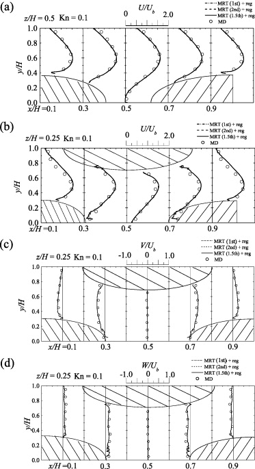
Suga and Ito (2011) considered the channel flows whose walls were 3D bumpy shapes to discuss the performance of the LBM for the three-dimensionally curved surfaces. Figure 21 shows the computational domain and schematic views of the 3D bumpy channel flow considered. As shown in figures 21(a) and (b), the matrices of hemisphere bumps were placed on the top and bottom walls in a staggered fashion. The radius of the hemisphere was R = 0.4H where H is the channel height and the pitch of the bumps. Periodic boundary conditions were applied to the streamwise (x ) and spanwise (z ) directions. To drive the fluid, the force was applied to the x-direction only. The estimated Knudsen number in the MD simulation was Kn = 0.1. The corresponding MRT LBM simulations were carried out on the 3D grids using the linear IDBBC with the regularization and Ψ 1 by the D3Q19 model. The grid size used was 100 × 100 × 100 .
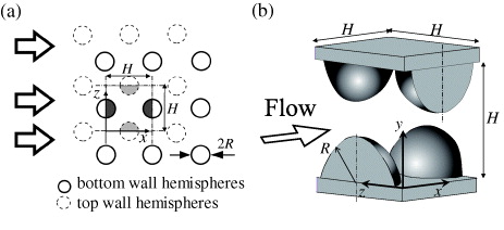
Figure 21. Computational domain of a 3D bumpy wall channel flow: (a) plane view of the computational domain and (b) schematic view of the flow field. Figures taken from Suga and Ito (2011). Copyright 2011, Tech Science Press.
Download figure:
Standard image High-resolution imageFigure 22 compares the velocity profiles at the symmetry plane, z/H = 0.5 (figure 22(a)), and an off-center plane, z/H = 0.25 (figures 22(b)–(d)). As discussed in the 2D flow cases, with the regularization procedure, it is clearly seen that all the slip-flow models show the same predictive tendency. Generally, the agreement between the MRT LBM and the MD simulation results is very satisfactory. The maximum discrepancy between the results is indeed up to 15% of the bulk velocity Ub . However, unlike the 2D flows, even with the regularization, somehow kinky profiles still can be seen near walls at some sections such as x/H = 0.1 and 0.9 in the symmetry plane (figure 22(a)). Also weak oscillations appear near the bottom wall at x/H = 0.3 and 0.7 in the plane of z/H = 0.25 (figures 22(b)–(d)). Since the flow field and characteristics are much more complicated than those of the 2D test flows, it may not be easy to dampen such near-wall kinks or oscillations by the regularization procedure even at Kn = 0.1. It is worth re-considering the interpolation scheme for the diffusive bounce-back boundary condition used in the study because its accuracy of the curvature representation in the tangential direction is first order.
Figure 22. Comparison of velocity profiles by the MRT LBM with the first-, 1.5th- and second-order slip flow IDBBC, the regularization and Ψ 1 in a 3D bumpy channel at Kn = 0.1: (a) streamwise velocity component at z/H = 0.5 , (b) streamwise velocity component at z/H = 0.25 , (c) vertical velocity component at z/H = 0.25 and (d) spanwise velocity component at z/H = 0.25 . Figures taken from Suga and Ito (2011). Copyright 2011, Tech Science Press.
Download figure:
Standard image High-resolution image
4. Conclusions
This paper summarizes the results of the studies of evaluation of the μ-flow LBMs in several 2D and 3D test flow cases. For the 2D cases, they are force-driven Poiseuille flows, Couette flows, a combined nanochannel flow, and flows in a nanochannel with a square- or triangular cylinder placed at the center region. The 3D cases are nano-mesh flows and flow through a 3D bumpy channel. The focused flows are mainly in the slip and a part of the transitional flow regimes at Kn < 1. The evaluated schemes of the μ-flow LBMs are the LBGK LBM and the MRT LBM with several combinations of the boundary conditions and the discrete velocity models.
By adding several models such as the kinetic boundary condition and the molecular mean free path correction to the LBE for micro-flows, it was confirmed that the LBMs fairly satisfactorily reproduced velocity profiles and slippage velocities at the walls of the Poiseuille and Couette flows in the regime at Kn < 0.1. The near-wall correction of the molecular mean free path improves the results particularly at Kn > 0.1. However, they failed to accurately reproduce the Knudsen-layer corrections even by a tailor-made wall function to correct the molecular mean free path near the wall.
Although the conventionally simpler D2Q9 and D3Q19 discrete velocity models of the LBM were less accurate compared with the D2Q21 and D3Q39 models, their deficiency was not significant in the complex flow fields. Indeed, the D2Q9 and D3Q19 models predicted comparable flow profiles with those by the D2Q21 and D3Q39 models in the 2D square cylinder flow and the 3D nano mesh flows. This suggests that retaining terms of the third order in the Hermite expansion and using a Gauss–Hermite quadrature of the third order to obtain the discrete velocity values are not significantly important for predicting general flow profiles in complex micro- and nano-flows.
The diffuse scattering wall boundary condition showed generally acceptable results in fully developed flows. The bounce-back/specular-reflection boundary model, however, performed worse with a fixed bridge coefficient particularly in the combined nanochannel flow. Hence, the bridge coefficient for the bounce-back/specular-reflection wall boundary model should have dependence on local flow quantities. To describe complex flow geometries, the diffuse scatter or diffusive bounce-back boundary condition is easy to combine with the interpolated boundary treatment. With the diffusive bounce-back boundary condition, the MRT LBM can be suitably incorporated with the slip-flow model proposed by the kinetic theory unlike in the LBGK LBM. However, the results of the 3D bumpy channel flow by the MRT LBM with the diffusive bounce-back boundary condition suggested that some more sophisticated treatments would be required to enhance the stability in the vicinity of the three-dimensionally curved surfaces.
Without the regularization process, the entire flow field prediction suffered unphysical momentum distribution around a bluff body. For complex flows, the regularization procedure was essential to stabilize the solution results. With the regularization procedure, the coefficients of the first- to second-order slip-flow models, which were used to determine the relaxation times of the MRT LBM with the diffusive bounce-back wall boundary condition, hardly affected the simulation results by the D2Q9/D3Q19 model. Since the regularization process enforced the system to be confined within the second-order Hermite moment space for the D2Q9/D3Q19 model, all the higher-order non-equilibrium contributions from both the numerical and physical processes were filtered out. It is thus considered that any difference caused by the slip-flow model is corrected along with the other higher-order contributions included in the LBE.
Acknowledgments
The author thanks his students: Messrs S Takenaka, T Ito, H Yasuoka, and colleagues: Dr S Hyodo, Dr T Kinjo, Dr M Kaneda, for their collaboration to the series of studies summarized in this paper. The author also thanks Dr X-D Niu of Doshisha University for his collaboration while X-DN was working for the research project: the Core Research for Evolutional Science and Technology (CREST) of Japan Science Technology Agency (no. 228205R) that supported the initial stage of this series of studies. This series of studies was also partly supported by the Japan Society for the Promotion of Science through a Grant-in-Aid for Scientific Research (B) (no. 18360050), the Yazaki Memorial Foundation for Science and Technology, the Tanigawa Foundation, the Sumitomo Foundation and the Steel Industry Foundation for the Advancement of Environmental Protection Technology, Japan.
Appendix.: Comments on the slippage velocity by the LBGK model
Luo (2011) pointed out that the slippage velocity by the LBGK model was dependent on both the relaxation time and the grid resolution and thus the slip velocity obtained by the LBGK model was a numerical artifact. However, the present author's view is different. In the LBGK LBM with the DSBC, it is required that r = 1 and τν = τq = τ ; then equation (29) reduces to

with Ny = H/δ x and  . When the velocity profile is assumed to be parabolic, the slippage velocity by the LBGK LBM with the DSBC models can be thus expressed by the quadratic equation of Kn. Due to the relation between Kn and the relaxation time
  , equation (A.1) shows that the slip velocity is dependent on the relaxation time and Ny. Yet, one can expect convergence of the slip velocity at a 'fixed Kn' with a large enough number of Ny . Therefore, it shows that the slippage velocity by the LBGK model is not necessarily grid dependent and we can obtain grid-independent solutions with a relatively large Ny . However, the slip velocity described by equation (A.1) is fixed for the given Kn and cannot be accommodated to the given second-order slip velocity boundary condition of equation (28) unlike the MRT model. This clearly shows another superior point of the MRT model over the LBGK model.
Note that since the relaxation time is rewritten as  , with a fixed Kn, τ increases when Ny increases. However, due to μ = (τ - 1/2)pδ t, the Reynolds number: ρ UH/μ becomes
  . With the Mach number Ma = U/cs , this only shows the well-known relation
  when the specific heat ratio is unity, which is the assumption in the isothermal LBM. Obviously, Re is totally independent of Ny in the LBGK LBM.