


ABSTRACT
Following the work of Dexter & Agol, we present a new public code for the fast calculation of null geodesics in the Kerr spacetime. Using Weierstrass's and Jacobi's elliptic functions, we express all coordinates and affine parameters as analytical and numerical functions of a parameter p, which is an integral value along the geodesic. This is the main difference between our code and previous similar ones. The advantage of this treatment is that the information about the turning points does not need to be specified in advance by the user, and many applications such as imaging, the calculation of line profiles, and the observer-emitter problem, become root-finding problems. All elliptic integrations are computed by Carlson's elliptic integral method as in Dexter & Agol, which guarantees the fast computational speed of our code. The formulae to compute the constants of motion given by Cunningham & Bardeen have been extended, which allow one to readily handle situations in which the emitter or the observer has an arbitrary distance from, and motion state with respect to, the central compact object. The validation of the code has been extensively tested through applications to toy problems from the literature. The source FORTRAN code is freely available for download on our Web site http://www1.ynao.ac.cn/~yangxl/yxl.html.
Export citation and abstract BibTeX RIS
1. INTRODUCTION
There is wide interest in calculating radiative transfer near a compact object, such as a black hole, a neutron star, or a white dwarf. The radiation is affected by various effects such as light bending or focusing, time dilation, Doppler boosting, and gravitational redshift of the strong gravitational field of compact objects. Considering these effects helps us not only to understand the observed results, and therefore to study these compact objects, but also to test the correctness of general relativity under strong gravity. A good example is the study of the fluorescent iron line in the X-ray band at 6.4–6.9 keV, which is seen in many active galactic nuclei, especially Seyfert galaxies (Laor 1991; Fabian et al. 2000; Müller & Camenzind 2004; Miniutti & Fabian 2004; Miniutti et al. 2004). The line appears broadened and skewed as a result of the Doppler effect and gravitational redshift; thus, it is an important diagnostic for studying the geometry and other properties of the accretion flow in the vicinity of the central black hole (Fabian et al. 2000). Another example is the study of the supermassive black hole (SMBH) in the center of our Galaxy. It has been comprehensively accepted that in the center of our Galaxy an SMBH with a mass of ∼4 × 10⁶ M☉ exists (Schödel et al. 2003; Gebhardt et al. 2000; Hopkins et al. 2008) and that its shadow may be observed directly in the radio band in the near future. Based on the general relativistic numerical simulations of the accretion flow, Noble et al. (2007) present the first dynamically self-consistent models of millimeter and sub-millimeter emission from Sgr A*. Yuan et al. (2009) calculated the observed images of Sgr A* with a fully general relativistic radiative inefficient accretion flow.
A natural way to include all of the gravitational effects is to track the ray following its null geodesic orbit, which requires fast and accurate computations of the trajectory of a photon in the Kerr spacetime. Fanton et al. (1997) proposed a fast code to calculate the accreting lines and thin disk images. Čadež et al. (1998) translated all integrations into Legendre's standard elliptic integrals and wrote a fast numerical code. Dexter & Agol (2009) presented a new fast public code, named geokerr, for computing all coordinates of null geodesics in the Kerr spacetime using Carlson's elliptic integrals semi-analytically for the first time. There are two computational methods often used in these codes: (1) the elliptic function method which relies on the integrability of the geodesics (Cunningham & Bardeen 1973; Cunningham 1975; Luminet 1979; Rauch & Blandford 1994; Speith et al. 1995; Fanton et al. 1997; Čadež et al. 1998; Li et al. 2005; Wu & Wang 2007; Dexter & Agol 2009; Yuan et al. 2009) and (2) the direct geodesic integration method (Fuerst & Wu 2004; Schnittman & Rezzolla 2006; Dolence et al. 2009; Anderson et al. 2010; Vincent et al. 2011; Younsi et al. 2012; Chan et al. 2013). Usually people regard the direct geodesic integration method as a better choice than the elliptic function method, for the direct geodesic integration method can deal with any three-dimensional accretion flow (Younsi et al. 2012), especially in radiative transfer problems which require the calculation of many points along each geodesic. The direct integration method is furthermore simpler and faster (Dolence et al. 2009). On the other hand, the elliptic function method is considered to be sufficient only for the calculation of the emission that comes from an optically thick, geometrically thin, axisymmetric accretion disk system. But we think that the elliptic function method based on the work of Dexter & Agol (2009) can, after some extensions, overcome these shortages and not only handle three-dimensional accretion flows readily, but also be more efficient, flexible, and accurate because it can compute arbitrary points on arbitrary sections for any geodesics. The speed of the code based on this approach is still very fast for many potential applications. While the direct geodesic integration method must integrate the geodesic from the initial position to the points of interest, the waste of computational time is inevitable.
We present a new public code for the computation of null geodesics in the Kerr spacetime following the work of Dexter & Agol (2009). In our code, all coordinates and the affine parameters are expressed as functions of a parameter p, which corresponds to Iu or Iμ in Dexter & Agol (2009). Using the parameter p as an independent variable, the computations are easier and simpler, and thus more convenient, mainly due to the fact that the information about the turning points does not need to be prescribed in advance as in Dexter & Agol (2009). Meanwhile, Yuan et al. (2009) demonstrated that the parameter p can replace the affine parameter as an independent variable in radiative transfer problems. We not only adopt this replacement, but also use it to handle more sophisticated applications. We extend the formulae of computing constants of motion from initial conditions to a more general form, which can readily handle cases in which the emitter or the observer has an arbitrary motion state and distance with respect to the central black hole. We reduce the elliptic integrals from the motion equations derived from the Hamilton–Jacobi equation (Carter 1968) to Weierstrass's elliptic integrals rather than to Legendre's, because the former are much easier to handle. Then, we calculate these integrals by Carlson's method.
The paper is organized as follows. In Section 2, we give the motion equations for null geodesics. In Section 3, we express all coordinates and affine parameters as functions of a parameter p analytically and numerically. In Section 4, we give the extended formulae for the computation of constants of motion. A brief introduction and discussion of the code are given in Section 5. In Section 6, we demonstrate the results of testing our code on toy problems from the literature. The conclusions and discussions are finally presented in Section 7. The general relativity calculations follow the notational conventions of the text given by Misner et al. (1973). The natural units are used throughout this paper, in which constants G=c=1, and the mass of the central black hole M is also taken to be 1.
2. MOTION EQUATIONS
Following Bardeen et al. (1972), we write the Kerr line element in the Boyer–Lindquist (B–L) coordinates (t, r, θ, ϕ) as

where

and a is the spin parameter of the black hole.
The geodesic equations for a free test particle read

where σ is the proper time for particles and an affine parameter for photons, uν is the four-velocity, and  represents the connection coefficients. Carter (1968) found that these equations are integrable under the Kerr spacetime and obtained the differential and integral forms of motion equations for the particles using the Hamilton–Jacobi equation. For a photon whose rest mass m is zero, the equations of motion have the following forms:


where


q and λ are constants of motion defined by

and where Q is the Carter constant, Lz is the angular momentum of the photon about the spin axis of the black hole, and E is the energy measured by an observer at infinity. The four-momentum of a photon can be expressed as

which is often used in the discussion of the motion of a photon.
From Equation (13) we know that if q = 0 and θ ≡ π/2, then Θθ ≡ 0. θ ≡ π/2 means that the motion of the photon is confined in the equatorial plane forever (Chandrasekhar 1983). Thus, the motion equations with integral forms now become invalid because Θθ = 0 appears in the denominator. We therefore need motion equations with differential forms.
From Equation (4) we have

where the subscript pm means "plane motion." Dividing Equation (6) by Equation (4) and integrating both sides, we obtain

Similarly, from Equations (7) and (4), we obtain

Spherical motion is another special case in which the photon is confined to a sphere and its motion can be described by the following equations: R ≡ 0 and dR/dr ≡ 0 (Bardeen et al. 1972; Shakura 1987). Thus, the motion equations with integral forms also become invalid because R = 0 appears in the denominator. Similarly, from Equation (5) we have

where the subscript sm means "spherical motion." Dividing Equation (6) by Equation (5) and integrating both sides, we have

From Equations (5) and (7) we have

From Equation (8), we introduce a new parameter p with the following definition to describe the motion of a photon along its geodesic (Yuan et al. 2009):

Because the sign in front of the integral is the same with dr and dθ, p is always nonnegative and increases monotonically as the photon moves along the geodesic. From the above definition, we know that r and θ are functions of p. In the next section, we give the explicit forms of these functions using Weierstrass's and Jacobi's elliptic functions.
3. THE EXPRESSION OF ALL COORDINATES AS FUNCTIONS OF p
3.1. Turning Points
From the equations of motion, we know that both R and Θθ must be nonnegative. This restriction divides the coordinate space into allowed (where R ⩾ 0 and Θθ ⩾ 0) and forbidden (where R < 0 or Θθ < 0) regions for the motion of a photon. The boundary points of these regions are the so-called turning points, and their coordinates rtp and θtp satisfy equations R(rtp) = 0 and Θθ(θtp) = 0. For a photon emitted at rini and θini, its motion is confined between two turning points  and
and  for a radial coordinate, and
  and
and  for a poloidal coordinate. If we assume
  and
and  , then we have
 ![$r_{{\rm ini}}\in [r_{{\rm tp_1}}, r_{{\rm tp_2}}]$](https://content.cld.iop.org/journals/0067-0049/207/1/6/revision1/apjs472591ieqn8.gif) and
and ![$\theta _{{\rm ini}}\in [\theta _{{\rm tp_1}}, \theta _{{\rm tp_2}}]$](https://content.cld.iop.org/journals/0067-0049/207/1/6/revision1/apjs472591ieqn9.gif) . Because
. Because  and
and  , if pr = 0 (or pθ = 0) at the initial position, we have R(rini) = 0 (or Θθ(θini) = 0); therefore, rini (or θini) must be a turning point and equal to one of
  and
and  (or
(or  and
and  ).
).
The radial motion of a photon can be unbounded, meaning that the photon can go to infinity or fall into the black hole. These cases usually correspond to the equation R(r) = 0 which has no real roots or  is less than or equal to the radius of the event horizon. We regard infinity and the event horizon of the black hole as two special turning points in the radial motion. A photon asymptotically approaches them but never returns from them. Thus,
  can be infinity and
  can be less than or equal to rh (here rh is the radius of the event horizon).
For the poloidal motion, there are also two special positions: θ = 0 and θ = π, i.e., the spin axis of the black hole. A photon with λ = 0 goes through the spin axis due to zero angular momentum and changes the sign of its angular velocity dθ/dσ instantaneously, and its azimuthal coordinate jumps from ϕ to ϕ ± π (Shakura 1987), implying that the spin axis is not a turning point. From Equation (13), we also know that 0 and π are not the roots of the equation Θθ(θ) = 0.
3.2. μ Coordinate
First, we use a new variable μ to replace cos θ, and Equation (23) can be rewritten as

where

Both R and Θμ are quartic, but the polynomial of Weierstrass's standard elliptic integral is cubic. We need a variable transformation to make R and Θμ cubic. We define the following constants for poloidal motion:


where  and introduce a new variable t,

Making the transformation from μ to t, the μ part of Equation (24) can be reduced to

where  ,
,  Using the definition of Weierstrass's elliptic function ℘(z; g2, g3) (Abramowitz & Stegun 1965) from Equation (31), we have t = ℘(p ± Πμ; g2, g3). Solving Equation (30) for μ, we can express μ as the function of p:

where

The sign in front of Πμ depends on the initial value of pθ, which is the θ component of the four-momentum of a photon, and

where ω is the period of ℘(z; g2, g3) and n = 0, 1, 2, .... The sign in front of Πμ can be "+" or "−" when pθ = 0.
From the above discussion, we know that one root of equation Θμ = 0 is needed in the variable transformation, namely,  . To avoid the complexity caused by introducing complex numbers, we always use the real root. Luckily, the equation Θμ = 0 always has real roots, but the same is not true for the equation R(r) = 0. For cases in which the equation R(r) = 0 has no real roots, we use Jacobi's elliptic functions sn(z|k2), cn(z|k2) to express r.
3.3. r Coordinate
If the equation R(r) = 0 has real roots, then  exists. We can define the following constants using
  :
:


and introducing a new variable t,

It is similar to μ, using t as an independent variable. We can reduce the r part of Equation (24) to the standard form of Weierstrass's elliptical integral

where  ,
,  Taking the inverse of the above equation, we get t = ℘(p ± Πr; g2, g3). Solving Equation (39) for r, we have

where

The sign in front of Πr also depends on the initial value of pr, which is the r component of the four-momentum of a photon, and

where ω is the period of ℘(z; g2, g3) and n = 0, 1, 2, .... The sign in front of Πr can be "+" or "−" when pr = 0.
If the equation R(r) = 0 has no real roots, we use Jacobi's elliptic functions to express r. Since the coefficient of r3 is zero, the roots of equation R(r) = 0 satisfy r1 + r2 + r3 + r4 = 0. Therefore, the roots r1, r2, r3, and r4 can be written as

Introducing two constants λ1 and λ2

which satisfy λ1 > 1 > λ2 > 0, and a new variable t,

we can reduce the r part of Equation (24) to Legendre's standard elliptic integral

where

Using the definition of Jacobi's elliptic function sn(z|k2) (Abramowitz & Stegun 1965), from Equation (47) we obtain  . Solving Equation (46) for r, we get the expression for r as a function of p

where

When the initial value of pr > 0, we have r = r−, and when pr < 0, we have r = r+. pr cannot be zero, otherwise the initial radial coordinate rini of the photon becomes one root of the equation R(r) = 0, which is the case that has been discussed above.
3.4. t and ϕ Coordinates and the Affine Parameter σ
In this section, we express the coordinates t, ϕ and the affine parameter σ as the numerical functions of the parameter p. All of these variables have been expressed as the integrals of r and θ in Equations (9)–(11) and (17)–(22). We achieve our goal if we can compute all of these integrals along a geodesic for a specified p. Making transformations from r and μ to a new variable t (defined by Equations (30), (39), and (46)), we compute these integrals under the new variable t. For simplicity, we use Fr(t) and Fθ(t) to denote the complicated integrands (see below) for r and θ, respectively.
First, we discuss the integral path, which starts from the initial position and terminates at the photon. If the photon encounters the turning points along the geodesic, then the whole integral path is not monotonic, as shown in Figure 1 for poloidal motion (radial motion is similar). In this figure, the projected poloidal motion of a photon in the r–θ plane is illustrated. The motion is confined between two turning points:  and
and  . The photon encounters the turning points three times. Obviously any section of the path that contains one or more than one turning point is not monotonic, such as paths CDE, EFP, etc. The path between any two neighboring turning points has the maximum monotonic length and the total integrals should be computed along each of them and summed.

Figure 1. Motion of a photon in the θ coordinate, which has been projected onto the r–θ plane. The motion is confined between two turning points μp1 and μp2. A, D, and F indicate the positions where the photon reaches the turning points and P indicates the position of the photon. The path between any two neighboring turning points (such as DA, DF) has the maximum monotonic length and the integrals of θ should be evaluated along each monotonic section and summed. The dotted (e.g., as CA, EF, and PF) and solid (e.g., DC and DE) lines represent the integral paths of I1 and I2 (see the text), respectively. The BC section is the integral path of I0, and one has  ,
,  ,
,  , etc.
Download figure:
Standard image High-resolution imageThere are four important points involved in the limits of these integrals, i.e.,  ,
,  , μini, and μp. These points are the μ coordinates of turning points, the initial point, and the photon position for a given p, respectively. The values of these points corresponding to the new variable t are
  ,
,  , tini, which can be calculated from Equation (30), and tp, which can be calculated from t = ℘(p ± Πμ; g2, g3) with a given p. Because the function t = t(μ) expressed by Equation (30) is monotonically increasing, we have
  and
and  .
.
We use Nt1 and Nt2 to denote the number of times a photon meets the turning points  and
and  for a given p, respectively, and define the following integrals (cf. Figure 1):

The integrals of θ in σ, t, and ϕ can be written as (cf. Figure 1)

where pθ is the θ component of the initial four-momentum of a photon. In order to evaluate the above expression, we need to know Nt1 and Nt2 for a given p. Similarly, if we define five integrals from Equation (31) as follows:

where W(t) = 4t3 − g2t − g3, we get the following identity:

Note that Nt1 and Nt2 are not arbitrary and are instead related to the initial direction of the photon in poloidal motion. For pθ > 0 (or pθ = 0 and  ), they increase as

For pθ < 0 (or pθ = 0 and  ), they increase as

For a given p, we find that one pair of Nt1 and Nt2 values that satisfies Equation (54) always exists. These values are the number of photons meeting the turning points. With Nt1 and Nt2, Equation (52) now can be evaluated readily.
For the r coordinate, the process is similar to that above. Nt1 and Nt2 also represent the number of times a photon meets the turning points  and
and  , respectively. Five integrals are defined as

where tp = ℘(p ± Πr; g2, g3) (or  when the equation R(r) = 0 has no real roots), and
  ,
,  , and tini are calculated from Equation (39) or Equation (46). Then the integrals of r in σ, t, ϕ can be written as

To get Nt1 and Nt2, we define p0, p1, and p2 from Equation (40) as

For a given p, we have

To get Nt1 and Nt2 from the above equation, one just needs to note that when pr > 0 (or pr = 0 and  ), they increase as

when pr < 0 (or pr = 0 and  ), they increase as

Similarly, for a given p, there is one pair of Nt1 and Nt2 values that satisfies Equation (58). With Nt1 and Nt2 values, Equation (56) can now be evaluated. In many cases, the number of times a photon meets the turning point in r is fewer than 2. Specifically, the number becomes zero when the equation R(r) = 0 has no real roots.
3.5. Reductions to Carlson's Elliptic Integrals
In previous sections, the four coordinates r, θ, ϕ, t and the affine parameter σ have been expressed as functions of p; many elliptic integrals need to be calculated using this routine. In this section, we reduce these integrals to standard forms and then evaluate them using Carlson's method as Dexter & Agol (2009) did.
First, we introduce two notations Jk(h) and Ik(h) with the following definitions:


where k is an integer. From Equation (8), we get one of the standard forms as

After having been reduced to J0, the forms of the integrals of r and θ in Equation (8) are exactly the same. Noting the definition of the parameter p, we have J0 = p. The radial integrals in Equation (9) are reduced to

where J0 has been replaced by p. The radial integrals in Equation (10) can be reduced to

where

Similarly, the radial integrals in Equation (11) have the following form:

where

When equation R(r) = 0 has no real roots, the integrals of r in σ, t, and ϕ can be written as


where

The integrals concerning μ in Equation (9) are reduced to

and tμ = σμ. The μ integrals in Equation (11) can be reduced to

where

Finally, we have

From Equations (61)–(72) the integrals that need to be calculated are J0, J1, J2, and I1, I−1, I−2. Now, we use Carlson's method to evaluate them. When equation 4t3 − g2t − g3 = 0 has three real roots denoted by e1, e2, and e3, Jk(h) can be written as (Carlson 1988)

where sh = sign[(y − h)k]. When equation 4t3 − g2t − g3 = 0 has one real root e1 and one pair of complex conjugate roots u+iv and u−iv, Jk(h) can be written as (Carlson 1991)

From Equations (30) and (39), we know that when  or
or  , t becomes ∞; thus, one limit of these integrals can be infinity.
The integrals Ik(h) can be reduced to Carlson's integrals directly (Carlson 1992)

where [p1, ..., pk] is a symbol used by Carlson (1992) to denote the elliptic integrals and has the following definition:

which can be evaluated by the formulae provided in Carlson (1988, 1989, 1991, 1992).
4. CONSTANTS OF MOTION
4.1. Basic Equations
In previous sections, we have expressed all coordinates as functions of a parameter p and discussed how to calculate them using Carlson's method, but before the calculation, one needs to specify the constants of motion and pr, pθ, which determine the signs in front of Πμ, Πr, Π0 and also how the number of turning points increases. In this section, we discuss how to compute λ and q and pr, pθ from  , which are the components of the four-momentum measured in the locally nonrotating reference frame (LNRF) and have been specified by the user.
First, following Bardeen et al. (1972), we introduce the LNRF observers or the zero angular momentum observer; the basis vectors of the orthonormal tetrad of the observers are given by

where

The covariant components of the four-momentum of a photon in B–L coordinates can be expressed as

where sr and sθ are the signs of the r and θ components. One can easily show that  ; namely (Shakura 1987)


From Equations (83) and (84) we have  and
and  , which determine the initial direction of the photon in the B–L system (cf. Equations (34) and (43)), thus determining how the number of turning points increases.
Solving Equations (82) and (85) simultaneously for λ, one obtains

Using λ and Equation (82), one obtains  . Using λ and E from Equation (84), one obtains the formula for calculating the motion constant q,

Thus, we have obtained the basic Equations (86) and (87) connecting λ, q and the components of the four-momentum  measured in the LNRF.
To prescribe  , one should note that it satisfies the following equation:

Thus there are only three independent components. Obviously the user can specify the four-momentum  directly in the LNRF or equivalently specify
  in any other reference frame of his/her own choice and then transform it into the LNRF using a Lorentz transformation, i.e.,
  , where
  is the transformation matrix. From Equations (86) and (87), we know that what one needs is just
  and
and

 should be specified by the user according to his/her own needs.4
As an example, in Figure 2, we show a group of null geodesics emitted isotropically from a particle moving around a black hole in a marginally stable circular orbit (rms) with a = 0.9375. The physical velocities of the particle with respect to the LNRF are  . The four-momentum
  are specified isotropically in the reference of the particle and then transformed into the LNRF by the Lorentz transformation expressed in Equation (90), i.e.,
  . With
  , the constants of motion are computed readily. The light bending and beaming effects are illustrated clearly in this figure.

Figure 2. Set of geodesics emitted isotropically from a particle that orbits around a black hole in a marginally stable circular orbit with a = 0.9375. x and y are pseudo-Cartesian coordinates in the equatorial plane of the black hole. The figure shows the light bending and beaming effects clearly. The circle in the center represents the boundary of the event horizon.
Download figure:
Standard image High-resolution imageIn the next section, we discuss how to compute  from impact parameters, which play a key role in imaging. For simplicity, we use the transformation expressed by Equations (90) and (91) if the observer has motion.
4.2. Calculation of Motion Constants from Impact Parameters
From the works of Cunningham & Bardeen (1973) and Cunningham (1975), we know that λ and q can be calculated from impact parameters, usually denoted α and β, which are the coordinates of the impact position of a photon on the photographic plate of the observer. The formulae provided by these authors read as follows (Cunningham & Bardeen 1973):


The above equations are valid only when the distance between the observer and the emitter is infinite and the observer is stationary. Practically speaking, the distance is not infinite, otherwise the integrals of coordinate t become divergent. When the distance is finite, the above formulae should be modified. We extend those formulae to general situations in which both the finite distance and the motion state of the observer are considered.
Considering the finite distance is very easy. One just needs to substitute the coordinates robs, θobs of the observer into Equations (86) and (87) in the calculation. Considering the motion state is more complicated, however. Obviously we can divide the motion states of the observer into two types. In the first one, the observer is stationary and in the second one the observer has physical velocities  with respect to the LNRF.
In the first instance, the observer is just an LNRF observer whose orthonormal tetrad is given by Equation (79), namely, e(a)(obs) = e(a)(LNRF) while in the second instance, the tetrad of the observer can be created by a Lorentz transformation, i.e.,  . Here,
  is given by Equation (91).
As shown in Figure 3, we can plot the image of a photon hitting the photographic plate. The plate is located in the plane determined by the basis vectors e(θ)(obs) and e(ϕ)(obs), and in which an orthonormal coordinate system α, β has been established. The basis vectors eα and eβ of the system are aligned with e(ϕ)(obs) and e(θ)(obs), respectively. All photons go through the center of the lens before hitting the plate. From this figure, one obtains the relationships between the impact parameters and  as follows:


Clearly, one can read off  ,
,  , and
, and  .
.

Figure 3. A photon hitting the photographic plate of an observer. The relationships between the impact parameters α, β and the components  of the four-momentum of the photon are derived from this event. Before hitting the plate, all photons go through the center of the lens. e(r)(obs), e(θ)(obs), and e(ϕ)(obs) are the contravariant basis vectors of the frame, and the basis vectors of α, β coordinates eα, eβ are aligned with e(ϕ)(obs), e(θ)(obs), respectively.
Download figure:
Standard image High-resolution imageTwo dimensionless factors, r and scal, have been multiplied to amplify the size of the image; otherwise it will be infinitely small since the distance D between the central compact object and the observer and the size of the target object L satisfy D ≫ L.
In the rest frame of the observer, spacetime is locally flat, and we still have

Using Equations (94), (95), and (96) and noting the signs of  , we obtain


Substituting Equations (97)–(99) into Equation (89), we get the functions  . We can then calculate λ and q from the impact parameters by using Equations (86) and (87).
One can verify directly that when robs → ∞, scal = 1, and  , Equations (86) and (87) reduce to Equations (92) and (93) immediately.
If the observer has motion, the image on the plate has a displacement in comparison with the image when the observer is stationary. The displacement is proportional to the observer's velocity and can be described by αc and βc, which are the coordinates of the image point of the origin of the B–L coordinate system on the photographic plate. Obviously, αc and βc satisfy the following equations:


Actually,  represents the projection of the spin axis of the black hole onto the plate. When
  , the above equations become αc = 0 and βc = 0. The region of the image on the plate therefore is [ − ΔL + αc, ΔL + αc] and [ − ΔL + βc, ΔL + βc], where ΔL is the half-length of the image.
4.3. Redshift Formula
The redshift g of a photon is defined by g = Eobs/Eem. From the above discussion, we know that  and
and  , where
  is the four-velocity of the emitter. We define

From Equation (82), we have  . Using Equation (81), g can be expressed as

where  are the coordinate velocities.
With  , the physical velocities of the emitter with respect to the LNRF
  can be written as (Bardeen et al. 1972)

with which the four-velocity of the emitter can be expressed as

Then g can be rewritten as (Müller & Camenzind 2004)

For an emitter moving in a Keplerian orbit, the formula for g reduces to

5. A BRIEF INTRODUCTION TO THE CODE
5.1. The Four Coordinates and the Affine Parameter Functions
We have expressed the four coordinates r, μ, ϕ, t and the affine parameters σ as functions of p. We denote them as follows:

In practical applications, we are interested in determining the original position where the photon was emitted or the paths traveled by the photon. To make the calculations effectively, all photons are traced backward from the observer to the emitter along geodesics, but not all photons that start from the observer go through the emission region one is interested in, and the tracing process is terminated when these photons either reach infinity or fall into the event horizon of a black hole.
Now we discuss how to determine the intersection of a geodesic with the surface of an optically thick emission region, assuming that the optical depth is so high that a sharp emission surface exits. The surface is smooth and continuous and can be described by an algebraic equation,

where x, y, and z are the pseudo-Cartesian coordinates defined by

In some special cases, the surface one considers may not remain stationary, and the surface equation becomes a function of time t, i.e., F(r, θ, ϕ, t) = F0. We introduce a function f(p) defined by

Then the roots of the equation f(p) = 0 correspond to the intersections of the geodesic with the target surface. Therefore, if the equation f(p) = 0 has no roots, the geodesic will never intersect with the surface. To solve this equation efficiently, we classify the geodesics into four classes denoted A, B, C, and D, according to their relationships with respect to a shell, as shown in Figure 4. The shell completely includes the emission region, and its inner and outer radii are rin and rout. We remind the reader that  and
and  are the turning points between which the radial motion of a photon is confined. Geodesics in the four classes satisfy the conditions—A:
  ; B:
; B:  ; C:
; C:  ; and D:
  , respectively, where rh is the radius of the event horizon.

Figure 4. Classifications of a set of null geodesics according to their relationships with respect to a shell. The inner and outer radii of the shell are rin and rout, respectively. The geodesics are divided into four classes, marked A, B, C, and D. Since the target object or the emission region is assumed to be completely included by the shell, only geodesics in classes B, C, and D have probabilities of intersecting with the target object or going through the emission region. The trajectories of the geodesics are schematically plotted and have been projected onto the r–θ plane. The central black region represents the black hole shadow.
Download figure:
Standard image High-resolution imageThe values of the parameter p corresponding to the intersections of the geodesic with the shell are denoted p1, p2, p3, and p4, which satisfy p1 < p2 < p3 < p4. Obviously, the roots of the equation f(p) = 0 may exist on intervals [p1, p2] and [p3, p4]. We use the Bisection or the Newton–Raphson method to search for the roots (Press et al. 2007).
Solving the radiative transfer equation in optically thin or thick media, one needs to evaluate integrations along the geodesic taking the affine parameter σ as an independent variable. Since we have taken p as an independent variable, we can replace σ by p to evaluate these integrals. From the definition of p, i.e., Equation (23), one has

and from Equations (4) and (5) one gets

From the above equations one immediately obtains

which converts the independent variable from σ to p in the radiative transfer applications (Yuan et al. 2009).
Finally, we discuss briefly the determination of a geodesic connecting the emitter and the observer (Viergutz 1993; Beckwith & Done 2005). We use αem and βem to represent the impact parameters of the geodesic connecting the observer and the emitter and pem to indicate the position of the emitter on the geodesic, in which the coordinates of the emitter are rem, μem, and ϕem. We have the following set of equations:


In principle, if we can solve this set of nonlinear equations simultaneously for pem, αem, and βem, the geodesic is determined uniquely. Therefore, the observer–emitter problem also becomes a root-finding problem. In our code, we use the Newton–Raphson method (Press et al. 2007) to solve these equations.
5.2. The Code
In this section we give a brief introduction to the code; a more detailed introduction is given in the README5 file. The code is named YNOGK (Yun-Nan Observatory Geodesics Kerr) and it was written in Fortran 95 using the object-oriented method. The code is composed of a couple of modules. For each module, a special function has been implemented and one can use all supporting functions and subroutines in that module by the command "use module-name." By adding corresponding modules into one's own code, one can easily develop new modules to handle special and more sophisticated applications.
Two modules named ell-function and B–L coordinate are the most important ones in YNOGK; the former includes supporting functions and subroutines for calculating Carlson's elliptic integrals and the R-functions. Many routines in this module come from geokerr (Dexter & Agol 2009) and Numerical Recipes (Press et al. 2007). The latter includes routines for computing all coordinates and the affine parameter functions: t(p), r(p), θ(p), ϕ(p), and σ(p). To call these routines, constants of motion and the components of the four-momentum  ,
,  ,
,  measured in an LNRF must be provided. These values can be computed by two subroutines named lambdaq and initial-direction in YNOGK. The former routine computes the constants of motion from the impact parameters, while the latter computes λ and q from the initial
  given in a reference K', which has physical velocities
  with respect to the LNRF. Of course, one can compute them by one's own subroutines according to one's needs. As discussed in Section 5.1, we present a module named pem-finding to search for the minimum root pem of the equation f(p) = 0; f(p) as an external function should be given by the user. In the module obs-emitter, we present routines to find the root of Equations (115)–(117) using the Newton–Raphson algorithm (Press et al. 2007). In the testing section of the code, this module has been used to determine the geodesic connecting the observer and the central point of a hot spot, which moves in the innermost stable circular orbit (ISCO). With the geodesic, the motion of the spot can be described easily. The results agree very well with those of previous works, in which a very different method was used to determine the motion of the spot, i.e., by tabulating the motion according to the time of the observer over one period (Schnittman & Bertschinger 2004; Dexter & Agol 2009).
All routines for computing Carlson's elliptic integrals have been extensively checked by the NIntegrate function in Mathematica. The original code for these routines comes from geokerr (Dexter & Agol 2009) and has been modified to adapt to our code. The original code for the computation of the R-functions comes from Numerical Recipes (Press et al. 2007). The same check has also been done for functions t(p), r(p), θ(p), ϕ(p), σ(p). When |α| and |β| ≲ 10−7, we let them be zero, since Carlson's integrals cannot maintain their accuracy. The treatment is the same for any other parameters if they take offending values. For some critical cases, special treatments also have been implemented.
5.3. Comparisons and Speed Tests
Our code has many points in common with the geokerr code of Dexter & Agol (2009). Both use Carlson's method to compute the elliptic integrals and use the elliptic functions to express all coordinates as functions of an independent variable, but the elliptic function we used is mainly Weierstrass's elliptic function ℘(z; g2, g3), which has a cubic polynomial, leading to a simpler root distribution and a reduction in the number of integrals. In our code, the four B–L coordinates r, θ, ϕ, t and the affine parameter σ are expressed as analytical or numerical functions of a parameter p, which corresponds to Iu or Iμ in Dexter & Agol (2009). With this treatment, one can compute the geodesics directly without providing any information about the turning points in advance, enabling one to track emission from a more sophisticated surface instead of being limited to a standard thin accretion disk. In the code testing section, we show the images of a warped disk, which has a curved surface.
Our strategy, i.e., expressing coordinates as functions of p semi-analytically, can be extended to compute the timelike geodesics directly, almost without any modifications. As mentioned in Dexter & Agol (2009), the calculations of the timelike geodesics involve many more cases. The main challenge is to specify the number of radial turning points for bounded orbits in advance, but our strategy does not require the specification of the number of turning points both in radial and poloidal coordinates in advance. Therefore, our strategy can be used naturally and effectively in the calculations of timelike geodesics even in a Kerr–Newmann spacetime.
In our code, we give the orthonormal tetrad of the emitter or the observer analytically, provided that the physical velocities with respect to the LNRF are specified. They may be useful in a Monte-Carlo-type radiative transfer code, which requires one to make frequent transformations between the references frames of the emitter and the B–L coordinate system (Dolence et al. 2009). As illustrated in Figure 2, emission in the reference frame of the emitter is isotropic, but from the perspective of the B–L coordinate system the emission is anisotropic due to the Doppler beaming effect.
Our testing results for various toy problems agree well with those of Dexter & Agol (2009). In Figure 5, we illustrate the projection of a uniform orthonormal grid from the photographic plate of the observer onto the equatorial plane of a black hole. The solid and dotted lines represent the results from our code and geokerr, respectively. The results agree with each other very well.

Figure 5. Projection of a uniform grid from the photographic plate of the observer onto the equatorial plane of a black hole. The inclination angle θobs is 60° and the black hole spin a is 0.95. The solid lines represent the results from our code and the dotted lines represent the results from geokerr. x and y are pseudo-Cartesian coordinates in the equatorial plane of the black hole.
Download figure:
Standard image High-resolution imageThe basic strategies used in YNOGK to compute elliptic integrals and functions are very similar to those used in geokerr. For example, we make it possible for YNOGK to compute the minimum number of R-functions and share them between routines. This strategy greatly improves the speed of our code, but there are still some differences between the two codes. First, we assemble r(p) and μ(p) into routines for computing t(p), ϕ(p) and σ(p); thus, the repeated calculations for the same integrals among those functions can be avoided. We provide a routine named ynogk to compute the four B–L coordinates and affine parameter simultaneously. We also provide two independent routines named radius and mucos to compute r(p) and μ(p), respectively. Secondly, YNOGK can save the values of variables used in calculations for the same geodesic but for a different p. These values can be used repeatedly.
YNOGK is almost as fast as geokerr in tracing radiations from an optically and geometrically thin disk because only one point, i.e., the intersection of the ray with the disk surface, needs to be calculated. For the radiative transfer calculations, in which many points are needed along each geodesic, YNOGK is a little slower than geokerr. The speed tests of a code are dependent not only on the applications but also on the environment of the running code. From the testing results of YNOGK, we expect that its speed is almost the same as that of geokerr in many other applications.
For more detailed introductions, we refer the reader to the README file. In the next section, we show the testing results of our code for toy problems.
6. THE TESTS OF OUR CODE
In this section, we present the testing results of our code for toy problems. The results not only demonstrate the validity of our code but also give specific examples of its utility. First, we show the image of a black hole shadow, in which the intensity represents the value of the affine parameter σ. In this example, we want to test the validity of the function σ(p). Then, we show the images of a couple of accretion disks and a rotationally supported torus; all of them are optically thick and have a sharp emission surface. The disks include the standard thin, thick, and warped disks. Next, we show the images of a ball orbiting around a Kerr black hole in a Keplerian orbit to illustrate the gravitational lensing effect. Then, we calculate the line profile of the Fe Kα line and the blackbody radiation spectra of a standard thin accretion disk around a Kerr black hole. In order to test the accuracy of the function t(p), we image a hot spot moving around a Kerr black hole in the ISCO for various black hole spins. We also calculate the spectrogram and light curves of the spot over one period of motion with various inclinations for a Schwartzschild black hole. Finally, we discuss the radiative transfer equation and its solution with which the radiative transfer process in a radiation-dominated torus around a black hole has been discussed. We provide images of the torus for optically thin and thick cases. The resolution of the images in this section is taken to be 801 × 801 pixels. Each pixel corresponds to a unique geodesic.
6.1. The Black Hole Shadow
As the first test of our code, we provide the image of a black hole shadow. We trace all photons backward from the photographic plate to the black hole along geodesics. The intensities of the image are taken to be the affine parameter σ evaluated from the observer to the terminations on the geodesic—either when the photon intersects the event horizon of the black hole or reaches a turning point and returns to the starting radius. The evaluations of the affine parameter outside the shadow are multiplied by a factor of 1/2. In Figure 6, we show the image from an edge-on view. We take the spin a to be 0.998, and the distance of the observer to be 106 rg, where rg is the gravitational radius.

Figure 6. Edge-on view of the shadow of a black hole with a near extremal spin (a = 0.998). The radial coordinate of the observer is 106 rg. The gray scale represents the value of the affine parameter σ evaluated from the observer to the terminated position—either at the black hole or re-emerging to the starting radius. Compare to Figure 2 of Dexter & Agol (2009). α and β are the impact parameters that describe the size and the position of the image on the photographic plate.
Download figure:
Standard image High-resolution imageTo evaluate the affine parameter σ from the function σ(p), we need ph, which is the value of parameter p corresponding to the event horizon and also the root of the equation r(p) = rh. We can get ph by evaluating the integral of r in the definition of p and do not need to solve this equation directly. We provide a routine named r2p to complete this evaluation.
6.2. Accretion Disks
Next, we present images of the accretion disks around a Kerr black hole, including the standard thin, thick, and warped disks. The imaging of the disks is usually the first step in calculating the line profiles of the Fe Kα line and the spectrum (Li et al. 2005). Usually, the pseudo colors of the image represent the redshift g or the observed flux intensity Iν of emission that comes from the disk.
In Figure 7, we show the image of a standard thin disk, the inner and outer radii of which are rms and 22 rg, respectively. The black hole spin a is 0.998 and the inclination angle θobs is 86°. The distance of the observer is 40 rg. The shape of the image is quite different from that observed from infinitely far away. We also illustrate the higher order images of the disk in this figure. Due to light bending and focusing, one can see the part behind the black hole and the bottom side of the disk. The color intensities represent the redshift g of emission that comes from the disk.

Figure 7. Image of a standard thin accretion disk whose inner and outer radii are rms and 22 rg, respectively. The black hole spin a is 0.998 and the inclination angle θobs is 86°. The radial coordinate of the observer is 40 rg. See Figure 6 of Beckwith & Done (2005) or Figure 4 of Dexter & Agol (2009) for comparison. The higher-order image is also shown. α and β are the impact parameters, and the intensity of the gray scale represents the redshift g of emission that comes from the surface of the disk.
Download figure:
Standard image High-resolution imageIn order to determine the intersection of the geodesics with the disk, we need to know the minimum root of the equation μ(p) = 0. We provide two routines named pemdisk and pemdisk-all to compute the root by evaluating the integral of μ in the definition of p. Using pemdisk, one can draw the direct image; while using pemdisk-all, one can draw the direct and higher-order images.
The surface of the thick disk has a constant inclination angle δ with respect to the equatorial plane (Wu & Wang 2007). To trace the thick disk, we need to solve the equation μ(p) = cos (π/2 − δ) to get p for the upper surface and μ(p) = cos (π/2 + δ) for the bottom surface; the roots of these two equations can also be computed with pemdisk and pemdisk-all. Since the surface particles of the disk no longer remain in the equatorial plane, they exhibit sub-Keplerian motion with an angular velocity given by (Ruszkowski & Fabian 2000)

where ΩK = 1/(r3/2 + a) is the Keplerian velocity and the parameter n is taken to be 3 here. Using Equation (107), we can calculate the redshift of the emission that comes from the disk. The images are shown in Figure 8 and they agree very well with Figure 10 of Wu & Wang (2007).

Figure 8. Images of a thick disk around a near extremal Kerr black hole (a = 0.998) for various inclination angles. The surface of the disk has a constant inclination angle δ with respect to the equatorial plane and δ is taken to be 30°. The inner radius is the marginally stable circular orbit rms and the outer radius is 20 rg. The inclination angles θobs are 5°, 30°, 55°, and 80° for panels (a), (b), (c), and (d), respectively. α and β are the impact parameters, and the intensities of the color represent the redshift g of emission that comes from the surface of the disk. Compare to Figure 10 in Wu & Wang (2007).
Download figure:
Standard image High-resolution imageWarped accretion disks are also very interesting objects in astrophysics (Bardeen & Petterson 1975; Wu & Wang 2007; Wang & Li 2012). Here, we discuss a very simple model of a warped disk, in which the disk is assumed to be optically thick and its surface can be described by (Wang & Li 2012)

where the parameters γ and β are defined by


where rin and rout are the inner and outer radii of the disk, and n1, n2, and n3 are the warping parameters. With the above equations, we get f(p) as follows:

With the minimum root of the equation f(p) = 0, we can image the warped disk. If the poloidal velocity  of the particle is nonzero, Equations (103) or (106) are used to calculate the redshift g (cf. Wang & Li 2012). The images of the warped disk are shown in Figure 9, in which the warping parameters n1 and n2 are nonzero, leading to disk warps along the azimuthal direction. For comparison, one can see Figure 3 of Wang & Li (2012), in which n1 is taken to be zero for simplicity. The shape of the disk from Wang & Li (2012) is quite different from that illustrated here.

Figure 9. Images of a warped accretion disk around a near extremal black hole (a = 0.998) viewed from different azimuthal angles. The inner and outer radii of the disk are rms and 50 rg, respectively. The observer's inclination angle θobs is 50°. The warping parameters are n1 = 4π, n2 = 4, and n3 = 0.95. The azimuthal angle γ0, which represents the viewing angle, is 0°, 45°, 90°, 135°, 180°, 225°, 270°, and 315° for the panels from left to right and top to bottom. For comparison, we show an image observed face-on in the final panel. The false color also represents the redshift g of the emission that comes from the surface of the disk. α and β are the impact parameters. We take the parameter n1 ≠ 0, leading to the warping of the disk along the azimuthal direction shown clearly in the final panel. This warping is the main difference compared to Figure 3 of Wang & Li (2012).
Download figure:
Standard image High-resolution image6.3. The Rotationally Supported Torus
In this section, we show the images of a rotationally supported torus. For simplicity, we give a brief introduction to the torus model here; for more detailed discussions we recommended papers by Fuerst & Wu (2004) and Younsi et al. (2012). The torus is assumed to be stationary and axisymmetric. Due to the balance of the centrifugal force, gravity, and the pressure force, the structure of the torus is stratified and the isobaric surfaces can be described by a set of differential equations (Younsi et al. 2012),


where


and Ω is the angular velocity. rk represents the radius at which the particle orbits with a Keplerian velocity. The index parameter n is crucial for regulating the angular velocity profile and adjusting the geometrical aspect ratio of the torus. ζ is an auxiliary parameter. In order to obtain the outer surface of the torus, one needs to specify the innermost radius of the torus. This radius is usually regarded as the intersection of the isobaric surface with the ISCO. Taking the innermost radius in the equatorial plane to be the initial condition, differential Equations (123) and (124) can now readily to be integrated. In Figure 10, we illustrate the images of the torus; the torus has the same parameters as in Figure 3 of Younsi et al. (2012) and the results agree with each other very well.

Figure 10. Images of a rotationally supported torus that is geometrically and optically thick. The torus parameters are n = 0.2 and rk = 12 rg. The black hole spin a is 0, 0.5, and 0.998 for the panels from top to bottom. The inclination angle θobs is 45° for the left column and 85° for the right column. The false color represents the redshift g of the emission that comes from the surface of the torus and the white areas represent the zero-shift regions. α and β are the impact parameters. Compare to Figure 3 of Younsi et al. (2012).
Download figure:
Standard image High-resolution image6.4. The Gravitational Lensing Effect
When the trajectory of a photon is close to a compact object, the photon's path will be bent or focused and multiple images will be observed. This effect is the so-called gravitational lensing effect due to a strong gravitational field. Here, this phenomenon is illustrated by a simple example in which a ball moves around a near extremal black hole (a = 0.998) in a Keplerian orbit. If the radius of the orbit is R0, then the angular velocity of the ball is  . The coordinates of the center of the ball become


Then, the function of the surface of the ball can be expressed as follows:

where r1 is the radius of the ball. The images observed from an edge-on view are illustrated in Figure 11. For different positions of the ball in its orbit, the image changes significantly and even becomes a ring as the ball moves to the back of the event horizon.

Figure 11. Gravitational lensing effect on the motion of a ball moving in a Keplerian orbit around a near extremal black hole (a = 0.998). The motion is observed from an edge-on view. The radii of the ball and the orbit are 5 rg and 20 rg, respectively. The central red region represents the black hole shadow. The azimuthal angles of the ball measured from the line of sight along the counter-clockwise direction are 0°, 90°, 150°, 160°, 180°, 195°, 210°, and 270° for panels (a)–(h), respectively. The pseudo color shows the redshift of the emission that comes from the surface of the ball. α and β are the impact parameters.
Download figure:
Standard image High-resolution image6.5. The Line Profiles of the Fe Kα Line
The calculation of line profiles is very easy, provided that the structure of the disk is specified (Bromley et al. 1997). For simplicity, we assume that the particles of the accretion flow have Keplerian motion and that the disk is geometrically thin and optically thick. The inner and outer radii of the disk are located at rms and 15 rg, respectively. The emission is monochromatic and its profile can be described by Dirac's δ function in the local rest frame of the flow

where n is the index of emissivity and is assumed to be 3. Since Iν/ν3 is invariant along a geodesic (Misner et al. 1973), we obtain the observed intensity Iobs = g3Iem, where g = νobs/νem is the redshift. Then, the observed flux density Fν at a frequency ν can be computed by integrating Iobs over the whole plate as in the following expression:

The observed intensities have been normalized in the computation. The results are shown in Figure 12, which agrees very well with Figure 3 of Čadež et al. (1998). From this figure, one can see that larger black hole spins lead to broadening at low frequencies, for the ISCO is closer to the event horizon, and gravitational redshift effects are more significant. Higher inclination angles lead to broadening at high frequencies for the Doppler beaming effect.

Figure 12. Theoretical line profiles of the Fe Kα line of a thin accretion disk for various black hole spins and inclination angles. The inner and outer radii of the disk are rms and 15 rg, respectively. Top row: a = 0.2; bottom row: a = 0.998. Left column: θobs = 10°; middle column: θobs = 30°; right column: θobs = 75°. The horizontal and vertical axes represent the frequency and flux of the line, respectively, and are normalized. The line profiles are in agreement with Figure 3 of Čadež et al. (1998).
Download figure:
Standard image High-resolution image6.6. The Blackbody Radiation Spectrum of a Keplerian Disk
In this section, we compute the spectrum of a Keplerian disk around a Kerr black hole to illustrate the effects of black hole spin and the observer's inclination angle on the observed profile of the spectrum (Li et al. 2005). Similarly, the disk is assumed to be geometrically thin and optically thick, and the radiation spectrum of the disk in its local rest frame is assumed to be an isotropic blackbody spectrum. We denote the effective temperature of the disk by Teff. Then, the radiation intensity at frequency ν can be written as

where h and kB are the Planck and Boltzmann constants, respectively. For blackbody radiation, the effective temperature is simply

where σSB is the Stefan–Boltzmann constant. Here, we do not consider the effect of the returning radiation of the disk on the spectrum; therefore F(r) is just the energy flux emitted from the disk's surface measured by a locally corotating observer. For the Keplerian accretion disk around a Kerr black hole, Page & Thorne (1974) presented the analytical expression for F(r), i.e.,

where  is the mass accretion rate, f is a function of r, a, rms, the seminal expression of which is given by Equations (15d) and (15n) of Page & Thorne (1974). With F(r), the effective temperature of the disk can be computed readily. Using the invariance Iν/ν3, one can get the observed intensity Iobs = g3Iem. The total observed flux density at frequency ν therefore is the integration of Iobs over the whole plate:

Then the photon number flux density is Nobs = F(νobs)/Eobs.
The results are plotted in Figure 13. Compared with Figure 5 of Li et al. (2005), we find that the basic features of the two figures are in agreement. For example, as shown in the top panel, we see that as the spin of the black hole increases the spectrum becomes harder. Physically, this effect is due to the fact that as the spin a increases, the system of the accretion disk has a higher radiation efficiency and a higher temperature. In the bottom panel of Figure 13, we can see that at the low-energy end, the flux density decreases as θobs increases. As explained by Li et al. (2005), this is caused by the projection effect. While at the high-energy end, the flux density increases as θobs increases. As pointed out by Li et al. (2005), this effect results from both Doppler beaming and gravitational focusing.

Figure 13. Effects of black hole spin (top) and inclination angle (bottom) on the spectrum of a standard thin accretion disk around a Kerr black hole. The inner and outer radii of the disk are rms and 30 rg, respectively, where rms is the radius of a marginally stable circular orbit.
Download figure:
Standard image High-resolution imageIn the top panel, there is a noticeable effect: even though we do not consider the returning radiation, the flux density increases as the spin increases at the low-energy end. Li et al. (2005) suggested that this effect is caused by the returning radiation. We propose that this explanation may not be correct and the effect is just caused by the simple fact that a higher spin leads to higher radiation efficiency and temperature.
6.7. The Motion of a Hot Spot
In order to test the validity of the function t(p) and illustrate the time delay effect in the Kerr spacetime, we image a hot spot that moves around a black hole in a prograde marginally stable circular orbit for various spins. We also compute the observed time-dependent light curve and spectra for a spot in retrograde ISCO around a Schwarzschild black hole for various inclination angles. The radius of the spot is Rspot = 0.5 rg. The emissivity of the spot is taken to be Gaussian in its rest frame (Schnittman & Bertschinger 2004), i.e.,

For the motion of the spot, one must consider the time delay effect and the azimuthal position of the spot when imaging the spot and calculating its spectra. In order to compute the time delay Δt for each geodesic starting from the photographic plate, a reference time tobs, which is taken to be the time required for a photon to travel from the central point of the spot to the observer, needs to be specified. Meanwhile, the position of the spot can be determined by its central coordinates (rms, μ = 0, ϕspot). Then, with the method discussed in Section 5 (i.e., the method for determining a geodesic connecting the observer and emitter with the given coordinates), we can determine the geodesic connecting the central point of the spot and the observer. With this geodesic, the reference time tobs can be calculated readily. Using tobs, we can easily calculate the time delay Δt for each geodesic, and Δt = tgeo − tobs, where tgeo is the time required for a photon to travel from the observer to the disk following the geodesic. With Δt and the position of the spot, we can compute the distance between the intersection of the geodesic with the disk and the center of the spot, i.e., |x − xspot|. Thus, the emissivity can be computed readily.
In Figure 14, we illustrate the images of the spot with different black hole spins. As the spin increases, the marginally stable circular orbit is closer to the event horizon of the black hole, and the time delay effect becomes significant. The image of the spot is strongly warped, especially when the spot moves to the back of the event horizon.

Figure 14. Images of a hot spot orbiting around a black hole in a prograde ISCO for different black hole spins. The spot lies in a standard thin accretion disk and its central point is fixed at the ISCO. We have extended the inner radius of the disk to the photon orbit rph, at which point the energy per unit rest mass of a particle is infinite. The photon orbit is also the innermost boundary of the circular orbit for particles (Bardeen et al. 1972). For the panels from left to right and top to bottom, the black hole spin a is 0.998, 0.5, 0, and −0.998, respectively. The inclination angle θobs is 85°. The false color represents the value of g − j(x), where g is the redshift of the emission that comes from the surface of the disk and j(x) is the emissivity of the spot.
Download figure:
Standard image High-resolution imageWhen an image is obtained, the redshift and Gaussian emissivity of all points on the spot can be computed. Repeating this procedure over one period of the motion gives a time-dependent spectrum. Integrating the spectrum over frequency, or equivalently over the impact parameters, gives the light curve. The spectrum and light curve are shown in Figure 15, and agree well with the results shown in Figures 6 and 7 of Dexter & Agol (2009).

Figure 15. Time-dependent spectrogram (panel (a)) and light curves (panel (b)) of a hot spot orbiting around a Schwarzschild black hole in a marginally stable circular orbit (6 rg) over one period. The inclination angle θobs is 60° for the spectrum. The gray scale in panel (a) represents the total sum of the emissivity j(x) of emission observed at the same time having the same redshift g. The gray scale has been normalized and the maximum is taken to be 1. Compare to Figures 6 and 7 of Dexter & Agol (2009).
Download figure:
Standard image High-resolution image6.8. Radiative Transfer
6.8.1. The Radiative Transfer Formulation
In this section, we briefly discuss radiative transfer in Kerr spacetime. One can find more detailed discussions from Fuerst & Wu (2004) and Younsi et al. (2012). It is well known that  , χ = ναν, and η = jν/ν2 are Lorentz invariants, where Iν is the specific intensity of the radiation and αν and jν are the absorption and emission coefficients at frequency ν, respectively. The radiative transfer equation reads (Younsi et al. 2012)

where τν is the optical depth at frequency ν and is defined by dτν = ανds and ds = −pμuμdσ, in which ds is the differential distance element of a photon traveling in the rest frame of the medium, σ is the affine parameter, pμ is the four-momentum of the photon, and uμ is the four-velocity of the medium. Then, the radiative transfer equation can be rewritten as (Younsi et al. 2012)

The solution of the above equation is (Younsi et al. 2012)

where the optical depth is

As discussed in Section 5.1, we can convert the independent variable from the affine parameter σ into the parameter p. Using σ = σ(p) and dσ = Σdp, we can rewrite the solution as the integration of the parameter p (Yuan et al. 2009)

where

With the above formulae one can deal with radiative transfer problems without considering the scattering contributions to the absorption and emission coefficients as was done by Yuan et al. (2009) and Younsi et al. (2012).
6.8.2. Radiative Transfer in Pressure-Supported Torus
In Section 6.3, we have discussed a rotationally supported torus and showed its images. When the torus is optically thick, only the emission that comes from the boundary surface is considered. When the torus is optically thin, all parts of the torus contribute to the observed emission. We need to consider the radiative transfer procedure along a ray inside the torus. To get the absorption and emission coefficients, we need to know the structure model of the tours, which determines the distributions of temperature, mass density, pressure, etc.
Firstly, we construct a model of the torus, in which the torus is a perfect fluid and its energy-momentum tensor is given by (Younsi et al. 2012)

where ρ is the mass density, P is the pressure,  is the internal energy, uα is the four-velocity of the fluid, and gαβ are the contravariant components of the Kerr metric. From the conservation law, namely,
  , we get the equation of motion of the fluid as follows (Abramowicz et al. 1978):

where the semicolon ";" represents the covariant derivative and uα; βuβ = aα is the four acceleration of the fluid. For a stationary and axisymmetric torus, we have at = 0, aϕ = 0, and ar, aθ given by (Younsi et al. 2012)


where  is the time component of the four-velocity and Ω is the angular velocity and takes the form of Equation (127). They satisfy the following equation

Since the torus is assumed to be radiation dominated, the pressure P can be regarded as the sum of the gas pressure Pgas and the radiation pressure Prad, and


where kB is the Boltzmann constant, μ is the mean molecular weight, mH is the mass of hydrogen, β is the ratio of gas pressure to the total pressure, and σ = π2k4/15ℏ3c3 is the blackbody emission constant. From the above equations, one finally obtains


Thus  , which implies that the state equation of the fluid is polytropic, therefore its internal energy is proportional to the pressure = P/(Γ − 1), and the equation of motion of the fluid (146) becomes

Substituting ∂αP = κΓρΓ − 1∂αρ and  into the above equation, one obtains

Introducing a new variable ξ defined by ξ = ln (Γ − 1 + κΓρΓ − 1), the above equation is simplified as

which implies that the vector n = (ar, aθ) in the r–θ plane can be regarded as the normal vector of the contours of the density ρ. Thus, if we use t = (dr, dθ) to denote the tangent vector of the contours, we have n · t = 0, or equivalently

If we use ds to denote the differential proper length of the tangent vector, we have

where grr and gθθ are the components of the Kerr metric and grr = Σ/Δ, gθθ = Σ. Solving Equations (157) and (158) simultaneously, we get a set of differential equations to describe the contours of density ρ


If we introduce an auxiliary variable ζ defined by  and substitute Equations (147) and (148) into the above equations, we get


which have exactly the same forms as Equations (123) and (124), where ψ1 and ψ2 are given by Equations (125) and (126). With these equations, the distributions of the mass density ρ of the torus now can be computed by evaluating the integral of ξ from the torus center r = rk, ρ = ρc to the location (r, θ) along a path C which is orthogonal to the density contours everywhere. The integral of ξ is

From Equations (152) and (153), one can get the total pressure and temperature distributions immediately with the given density ρ.
Knowing the structure model of the torus, the absorption and emission coefficients are now readily specified. We use these coefficients to discuss the radiative transfer process inside the torus. Using the above torus model, we give two examples of radiative transfer applications.
Firstly, we consider a rather simple case in which the torus is optically thin. The emissivity is taken to be proportional to the mass density ρ, i.e., jem∝ρ, and is independent of the frequency ν. The absorption coefficient αν is simply assumed to be zero. The torus parameters are n = 0.21 and rk = 12 rg. The black hole spin a is 0.998. The ratio of gas pressure to total pressure β is 2.87 × 10⁻⁸. In Figure 16, we show images of the torus, which is optically thin and radiation pressure dominated. We see that the emission mainly comes from the central region of the torus where the density is higher. As the inclination angle of the observer increases, the frequency shift of the emission from the Doppler boosting becomes larger. In this figure, the false color represents the observed intensities of the emission, showing that the approaching side of the torus is brighter than the receding side, especially at higher inclination angles.

Figure 16. Images of an optically thin torus dominated by radiation pressure. The inclination angles of the observer are 15°, 30°, 45°, 60°, 75°, and 90° for the panels from left to right and top to bottom. The black hole spin a is 0.998, and the ratio of gas pressure to total pressure β is 2.87 × 10⁻⁸. The torus parameters are n = 0.21 and rk = 12 rg. The brightness of each pixel represents the observed intensity integrated along a geodesic ray at a given frequency and has been normalized; the maximum for each panel is the same and equal to 100. α and β are the impact parameters.
Download figure:
Standard image High-resolution imageSecondly, we mimic a more realistic case, namely, thermal free–free emission and absorption, in which the torus is semi-opaque. The emission and absorption coefficients of the torus for a photon with energy E0 are given by (Younsi et al. 2012)


where Θ = kBT,  and B1 are the normalization constants, ne is the electron number density and ne = ρ/μmH, σT is the Thompson cross-section. The observed intensity images of the optically thick and semi-opaque torus are plotted in Figure 17. These images are quite different from those of an optically thin torus. The emissivity now depends on the temperature, which decreases toward the outer surface of the torus, leading to the limb darkening phenomenon. When the rays are nearly tangential to the layers of the torus, they travel a longer distance and go through the outer (colder) layers. On the other hand, when the rays are perpendicular to the layers of the torus, they travel a shorter distance and go through the inner (hotter) layers. Consequently, the observed intensity at lower inclination angles becomes much brighter than that at higher inclination angles (Younsi et al. 2012).

Figure 17. Images of an optically thick and semi opaque torus. The inclination angles are 15°, 30°, 45°, 60°, 75°, and 90° for the panels from left to right and top to bottom. The black hole spin a is 0.998, and the ratio of gas pressure to total pressure β is 2.87 × 10⁻⁸. The torus parameters are n = 0.21 and rk = 12 rg. The brightness of each pixel represents the observed intensity integrated over the entire spectrum. The intensity has been normalized, and the maximum of each panel is the same and equal to 100. α and β are the impact parameters.
Download figure:
Standard image High-resolution image7. DISCUSSION AND CONCLUSIONS
Following Dexter & Agol (2009), we have presented a new public code called YNOGK for the fast calculation of null geodesics in a Kerr spacetime. The code is written in Fortran 95 and is composed of a couple of modules. In this code, the object-oriented method has been used to ensure that the modules can be integrated with pre-existing code libraries. In YNOGK, the B–L coordinates r and μ have been expressed as analytical functions of the parameter p. In these expressions, Weierstrass's and Jacobi's elliptic functions ℘(z; g2, g3), sn(z|k2) and  are used, since reducing to Weierstrass's standard integrals are much easier, and only one real root of the equations R(r) = 0 and Θμ = 0 is required. The B–L coordinates t, ϕ and the affine parameter σ have been expressed as numerical functions of p. For a given p, the number of times a photon reaches the turning points both in radial and poloidal motions is uniquely determined and need not be specified by the user.
In addition to p, the coordinates r, μ (or θ) can also be taken as independent variables (Dexter & Agol 2009). The main reason for using p is that one ignore turning points, as has been done in the inner routines of our code. This virtue is convenient for a person who is not familiar with, or has no interest in, the details of the calculation of a geodesic in the Kerr spacetime. Another reason is that the value of p that corresponds to the termination of the geodesic—either at infinity or at the event horizon—is finite. Thus, it is easier to handle p than r. In our code, r and μ can also be taken as an independent variable. We provide a routine named geokerr, which can take r or μ as an independent variable. However, the number of turning points should be prescribed by the user.
With the expressions for all the coordinates and the affine parameter as functions of p, the ray-tracing problem, which determines the intersection of the ray with a target object, now becomes a root-finding problem. The function f(p) that describes the surface of the target object needs to be given by the user and the roots of the equation f(p) = 0 correspond to the intersections. We provide a module named pem-finding to search for the minimum root of this equation by the Bisection or the Newton–Raphson method. In addition, the observer–emitter problem can also be converted into a root-finding problem, which requires one to solve a set of nonlinear equations. A module named obs-emitter, based on the Newton–Raphson method to solve these equations, is provided in our code. The routines in this module return the solution, provided that the coordinates of the emitter, rem, θem, and ϕem, are given.
We present a new set of formulae to compute the constants of motion λ and q from initial conditions. These formulae can be regarded as extensions of the work of Cunningham & Bardeen (1973). Our formulae are adaptable and can be used to handle more sophisticated cases, in which the state of motion and the finite distance of the observer or the emitter with respect to the black hole are considered. One may find it convenient when dealing with problems in which the emitter has motion and is close to the vicinity of a black hole, e.g., the self-irradiation process in the inner region of a disk.
The code has been tested extensively with various toy problems from the literature. The results agree well with previous works. The comparisons with geokerr from Dexter & Agol (2009) also have been presented.
Finally, we point out that the strategy discussed in this paper can be naturally extended to the calculation of the timelike geodesics almost without any modification. Especially for the timelike-bounded orbits, the number of turning points both in poloidal and radial coordinates can be arbitrary. Extending this strategy to calculate the timelike geodesics in a Kerr–Newmann spacetime is complete and the results are under preparation.
We acknowledge financial support from the National Basic Research Program of China (973 Program 2009CB824800), the National Natural Science Foundation of China 11163006 and 11173054, and the Policy Research Program of the Chinese Academy of Sciences (KJCX2-YW-T24). We also thank the anonymous referee for very creative and helpful comments and suggestions that much improved both our work and the paper.
Footnotes
- 4
When a reference frame K' has physical velocities
 with respect to an LNRF, the general Lorentz transformation matrix has six independent parameters, i.e., , where θi are the angles between the corresponding spatial basis vectors of the two references. If θi = 0, the matrix can be written as follows (Misner et al. 1973):
where
, and its inverse form
- 5


![$\gamma =[1-(\upsilon _r^2+\upsilon _{\theta }^2+\upsilon _{\phi }^2)]^{-1/2}$](https://content.cld.iop.org/journals/0067-0049/207/1/6/revision1/apjs472591ieqn67.gif)

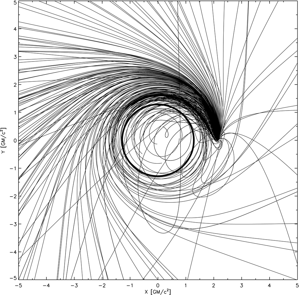
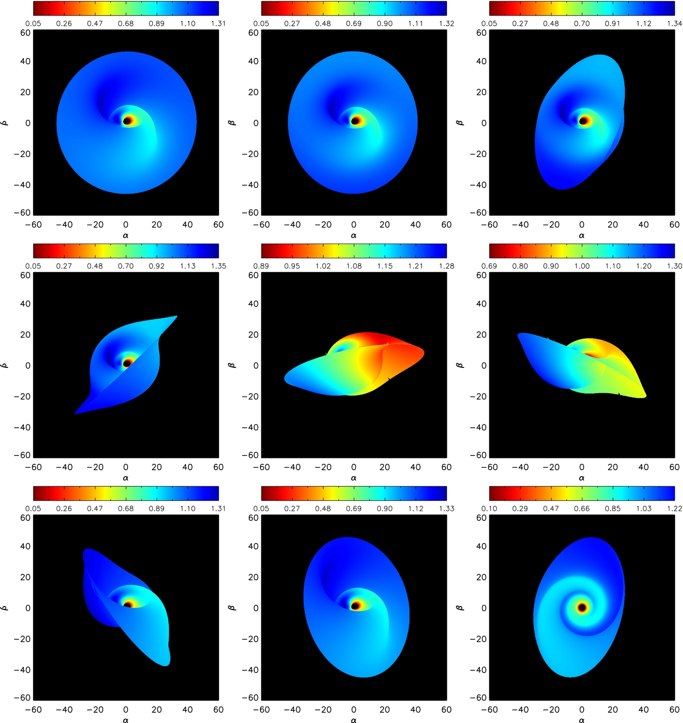