


ABSTRACT
We present fully sampled 38'' resolution maps of the CO and 13CO J = 2–1 lines in the molecular clouds toward the H ii region complex W3. The maps cover a 2 0 × 167 section of the galactic plane and span −70 to −20 km s−1 (LSR) in velocity with a resolution of ∼1.3 km s−1. The velocity range of the images includes all the gas in the Perseus spiral arm. We also present maps of CO J = 3–2 emission for a 05 × 033 area containing the H ii regions W3 Main and W3(OH). The J = 3–2 maps have velocity resolution of 0.87 km s−1 and 24'' angular resolution. Color figures display the peak line brightness temperature, the velocity-integrated intensity, and velocity channel maps for all three lines, and also the (CO/13CO) J = 2–1 line intensity ratios as a function of velocity. The line intensity image cubes are made available in standard FITS format as electronically readable files. We compare our molecular line maps with the 1.1 mm continuum image from the BOLOCAM Galactic Plane Survey (BGPS). From our 13CO image cube, we derive kinematic information for the 65 BGPS sources in the mapped field, in the form of Gaussian component fits.
Export citation and abstract BibTeX RIS
1. INTRODUCTION
The bright radio continuum source W3 was first cataloged by Westerhout (1958) in his survey of the galactic plane at 1390 MHz with an angular resolution of 057. The galactic longitude of W3 is l = 134°, at which our line of sight crosses the Perseus spiral arm at a distance of about 2 kpc. There have been many studies of radio continuum emission toward W3, which show an extended (∼30'–60') diffuse low-brightness component and several compact radio sources with complex structure and high emission measures. The radio continuum is dominated by thermal bremsstrahlung from ionized gas. The compact sources are H ii regions ionized by very luminous O stars, which indicate that W3 is the site of vigorous recent and continuing star formation. Spectroscopic observations of the ionized gas confirm the presence of compact, dense young H ii regions through detection of radio recombination lines, which provide the radial velocities of the ionized gas. One supernova remnant, HB3, has been identified by nonthermal radio and X-ray emission, lying at slightly lower galactic longitude than W3 (Landecker et al. 1987; Urosevic et al. 2007).
Many studies of the associated atomic and molecular interstellar gas in the direction of W3 have been published. The H i distribution and the 1.4 GHz radio continuum were mapped with ∼1' angular resolution by Normandeau et al. (1997) as part of the Canadian Galactic Plane Survey (CGPS; Taylor et al. 2003). The 12CO J = 1–0 line was mapped by Heyer et al. (1998) in the FCRAO Outer Galaxy Survey. A detailed analysis of the molecular data was made by Heyer & Terebey (1998). Carpenter et al. (2000) presented 13CO J = 1–0 data for regions containing IRAS point sources, and cataloged 19 stellar clusters embedded in the molecular gas over the W3/W4/W5 H ii region complex. Recently, images of the CO J = 3–2 emission made with the James Clerk Maxwell Telescope (JCMT) over an area comparable to that in this paper have been published by Polychroni et al. (2010). The data for the J = 2–1 lines which we present in this paper therefore fill in an important part of the picture of CO emission from the W3 molecular cloud, complementing both the J = 1–0 and J = 3–2 maps with similar areal coverage and angular resolution, and with superior sensitivity. The three rotational lines together will give stronger constraints on cloud models than any single transition by itself.
Large area maps with high angular resolution and high sensitivity in the infrared have been obtained through Spitzer programs including Ruch et al. (2007) and Polychroni et al. (2010). These data sets show the distribution of dust and polycyclic aromatic hydrocarbon emission, as well as shocked or UV-excited H2, but the wide bandwidth of the filters makes it difficult to separate the various emission components, and kinematic information is not possible. Likewise, the BOLOCAM Galactic Plane Survey (BGPS; Aguirre et al. 2011; Rosolowsky et al. 2010) at 1.1 mm wavelength reveals the long wavelength dust continuum with ∼30 mJy beam−1 rms sensitivity and 33'' angular resolution over the W3 region, but without velocity information.
X-ray images of the W3 region from the Chandra telescope have revealed dozens of point sources which are identified as lower-mass young stars, too cool to produce ionizing photons but still in active stages characterized by strong X-ray flares. These data have been discussed by Feigelson & Townsley (2008) in terms of the young stellar clusters within the molecular cloud. An extensive review of star formation in the W3/W4/W5 region is in Megeath et al. (2008). Taken together, the body of observations shows that the W3 region and its neighbors W4 and W5 are outstanding examples of a variety of stellar–interstellar feedback mechanisms. Prior generations of stars formed in W5 and W4 have likely triggered star formation in the W3 molecular cloud (e.g., Oey et al. 2005), and the resulting massive stars show evidence of influencing the remaining molecular gas. Given its relative proximity to the Sun and location in the outer Galaxy, the W3 cloud is a worthy target for improved studies of the molecular component and its relationship to current star formation in the entire region.
In this paper we present basic data for the W3 region, as part of a program to map selected galactic molecular clouds. (Results for the W51 region were presented by Bieging et al. 2010.) Since CO is both abundant and readily excited under typical cloud conditions, the lower-J rotational lines are an excellent choice to measure the spatial distribution and physical properties of molecular clouds over large areas of the sky. This cloud mapping program uses primarily the J = 2–1 rotational emission lines of two carbon monoxide isotopologues as tracers for the interstellar gas. No single tracer gives a complete representation of interstellar matter, but emission from the CO molecule has several advantages for determining an overall picture of molecular clouds. The J = 2 level of CO is ∼16.6 K (EJ/k) above ground and the critical density, ncrit, of the J = 2 level is 6 × 103 cm−3 for a kinetic temperature of 10 K (and summing over all collision rates connecting with the J = 2 level). The J = 2–1 transition will be readily excited throughout the bulk of any galactic molecular cloud, either by collisions in the denser parts or by radiative trapping in the regions with densities <ncrit. Although the emission from 12C16O, the most abundant isotopologue, may often be optically thick, the 13C16O isotopologue is lower in abundance by a factor of ∼50, so it is a useful tracer of total molecular column density. By comparing the line intensities of the two CO isotopologues along a given line of sight, together with spectra of other CO lines such as J = 1–0 and 3–2, the gas temperature, column density, and volume density may be constrained.
For the W3 cloud, we also obtained maps of the CO J = 3–2 line over a smaller part of the field mapped in the J = 2–1 lines. The J = 3–2 line has a critical density of 1.7 × 104 cm−3 at 10 K, and the upper state energy is at EJ/k = 33 K, so emission from this transition indicates warmer or denser gas than does the J = 2–1 line. Comparing the two transitions then allows some further constraints on the physical state of the molecular gas, in addition to the constraints from the J = 2–1 isotopologues.
This molecular cloud mapping program has several scientific goals, including the characterization of cloud structure and dynamics; and the identification of star-forming clumps through comparison with results from large area maps at other wavelengths, e.g., from Spitzer. Another goal is to provide "finding charts" of interesting molecular features for study with high angular resolution using aperture synthesis arrays such as CARMA. The need for such finding charts is evident when one considers that if CARMA were used to create a fully sampled mosaicked map of the W3 region presented here in the CO J = 2–1 line, more than 100,000 separate pointing centers would be required.
2. OBSERVATIONS AND DATA REDUCTION
Observations were made with the Heinrich Hertz Submillimeter Telescope (HHT) on Mt. Graham, AZ, at an elevation of 3200 m. The J = 2–1 lines of the CO isotopologues 12C16O (hereafter CO) and 13C16O (hereafter 13CO) were mapped over a 200 × 167 field covering the galactic coordinate ranges l = 1325 to 1345, b = 0° to +167. Observations were carried out in several observing sessions from 2005 June to 2008 April. For the observations through 2006 November, the receiver was the facility single-polarization, double-sideband superconductor–insulator–superconductor (SIS) mixer for the 1.3 mm wavelength band, which gave typical system temperatures in the range 300–500 K (converted to a single-sideband (SSB) scale). Beginning in 2006 December, a receiver employing a prototype ALMA Band 6 sideband separating mixer with dual orthogonal polarizations (Lauria et al. 2006) was used for the mapping program. This receiver permitted simultaneous observations of the CO and 13CO J = 2–1 lines in the upper and lower sidebands, respectively, with typically 15–17 dB of sideband rejection, thereby significantly improving the calibration accuracy and stability of the spectral intensity scales. Typical system temperatures with this receiver were between 180 K and 250 K (SSB), depending on weather conditions and source elevation.
We also mapped the CO J = 3–2 emission line over a limited region, covering 30' × 20' around the W3 Main and W3(OH) H ii region complexes (field center at l = 13375, b = +1167). The receiver was a seven-beam focal plane array of double-sideband heterodyne mixers (Groppi et al. 2003). The beam efficiency of the array elements was 0.50 ± 0.05 and the angular resolution was 24''. The velocity resolution of the spectra was 0.87 km s−1 for the J = 3–2 line maps. The CO J = 3–2 data were obtained at a single epoch, on 2006 April 12 and 13.
Data were taken by the "on-the-fly" (OTF) method, where the telescope was scanned in a boustrophedonic pattern in galactic longitude at a scan rate of 10'' s−1, with spectra sampled every 0.1 s. In subsequent processing, the data were smoothed by four samples or 0.4 s, corresponding to a telescope motion of 4'' per spectrum. The beam size at the CO J = 2–1 observing frequency is 32'' (full-width at half-maximum (FWHM)) so this choice of spatial sampling does not cause any significant loss of angular resolution in the scan direction. A raster of lines with 10'' spacing in latitude or ∼0.3 of the beam FWHM was observed in this way. The telescope resolution is well sampled in both coordinates with this choice of OTF mapping parameters. The field to be mapped was divided into 8 × 5 subfields, each 15' × 20'(l × b) in size, plus a small overlap. Each subfield was observed at least once in each of the two CO isotopologues. Total scanning time per subfield was therefore 3.0 hr, plus ∼30% overhead for telescope slewing and measurement of reference spectra after every other row. Subfields were re-observed in whole or part if weather conditions resulted in excessively high noise levels. Two subfields, in the top right and bottom right corners of the 8 × 5 grid, were omitted due to time constraints and because the CO emission is negligible in those regions (as shown in Heyer & Terebey 1998). The CO J = 3–2 line was mapped in the same way, with the same OTF scanning parameters. The grid spacing was also 10'', or about 40% of the telescope diffraction-limited resolution. Since the array receiver sampled multiple positions on the sky during each scan, the field was well sampled when the individual focal plane elements were combined in the final map.
For the observations prior to 2006 November, spectra were measured with an acousto-optic spectrometer (AOS) having a frequency resolution of 1 MHz (corresponding to a velocity resolution of 1.3 km s−1 for the CO J = 2–1 line), and a total bandwidth of 1 GHz. The AOS channel spacing and frequency were calibrated regularly to ensure the accuracy of the velocity scale in the measured spectra. We estimate that the calibration accuracy was maintained to 10% of the spectral channel width, or 0.13 km s−1 in velocity.
For observations after 2006 November, we used a new filterbank spectrometer instead of the AOS, to record both the CO and 13CO data simultaneously. Each of the two J = 2–1 lines was measured with 1024 filters of 1 MHz bandwidth, giving a total spectral coverage and resolution essentially the same as with the AOS. The J = 3–2 spectra were taken with the same filterbank spectrometer, but configured to provide seven spectra each with 256 channels of 1 MHz bandwidth, one for each of the seven elements of the focal plane array.
The telescope pointing accuracy was checked at the start of each observing period by measuring the CO J = 2–1 emission from the carbon star V384 Per or the M-type Mira R Cas, both of which have strong CO emission lines from their circumstellar molecular envelopes. These objects are good pointing calibrators for the W3 field because the stellar emission is compact and centered on the well-known positions of the stars, which are only about 20° from the W3 field. A five-point cross pattern centered on the star was measured and the integrated line intensities at the five positions were fitted to determine the pointing corrections in azimuth and elevation. These corrections were generally <5''. The pointing was checked and corrected about every 2 hr throughout each observing run, so the pointing errors during the OTF mapping should be <5''.
The intensity scale was determined with the standard method of Kutner & Ulich (1981) by comparing an ambient temperature load with on-sky spectra near the target field, to give the spectral line intensity on the T*A scale. For the double-sideband mixer receivers, the response was assumed to be equal in the two sidebands in deriving the spectrometer intensity scale. For the sideband separating mixer receiver, the sideband rejection was measured each time the receiver was tuned. We observed a standard position, W3(OH) (R.A. (J2000) =  , decl. (J2000) = 61°52'24
 4, or l = 1339475, b = 10642), which is from the Wang et al. (1994) list of spectral line calibrators, at least once in each observing session to calibrate the main beam brightness temperature scale. The main beam brightness temperatures for W3(OH) were derived from the measured main beam efficiency, which was determined by observations of planets. For the CO J = 2–1 line frequency (in the receiver upper sideband), the measured efficiencies were 71% and 76% for the two orthogonal polarizations of the ALMA prototype receiver, and for the 13CO line (in the lower sideband) the values were 74% and 72%. From these efficiency calibrations, we adopted main beam brightness temperatures integrated over the velocity range −70 to −20 km s−1, of 277 K km s−1 for the CO J = 2–1 line and 107 K km s−1 for the 13CO J = 2–1 line for the HHT pointed on W3(OH). From the internal consistency of repeated measurements, we estimate that the adopted line-integrated intensities are accurate to better than ±10%. The intensity scale (in T*A) of each OTF observation was scaled by the associated W3(OH) measurements to place all of the mapping data on the same main beam brightness temperature scale. Spectra of W3(OH) for the two J = 2–1 isotopologue lines and the CO J = 3–2 line are shown in Figure 1, plotted on our measured main beam brightness temperature scale.
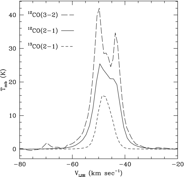
Figure 1. Spectra of the standard source W3(OH), used to set the main beam brightness intensity scale for the W3 maps. Telescope resolution is 32'' (FWHM) for the J = 2–1 lines and 24'' (FWHM) for the J = 3–2 line.
Download figure:
Standard image High-resolution imageThe main beam brightness temperature scale for the CO J = 3–2 map was determined by scaling the measured spectrum extracted from our OTF map at the position of W3(OH), to match the SSB-calibrated spectrum of Wang et al. (1994). Comparing their spectrum with spectra extracted from our map, we find a discrepancy in the detailed shape of the spectra. The best match in spectral profiles was for a position on our CO J = 3–2 map offset by ∼ + 10'' in galactic latitude from the nominal position of W3(OH) used by Wang et al. (1994). This offset is within the combined pointing uncertainties of their data (taken on the Caltech Submillimeter Observatory) and ours.
All of the OTF data were processed in the CLASS software package of the Grenoble Astrophysics Group. A linear baseline was removed from each spectrum and the data for each spectral channel were convolved to a square grid in galactic longitude and latitude, with a 10'' grid spacing in both coordinates. The gridding algorithm uses a circular Gaussian weighting function with an FWHM of 0.3 × (beam FWHM), to convolve the OTF-sampled spectra onto the regular grid points. The gridding thereby increased the effective angular resolution by a factor of (1 + 0.32)1/2 = 1.044.
The resulting data cubes were transferred to the MIRIAD software format (Sault et al. 1995) for subsequent processing and analysis. To facilitate the comparison of CO and 13CO lines (for example, to calculate line ratios at each pixel), we used the MIRIAD task regrid to resample the data cubes on the velocity axis by third-order interpolation. We chose to sample velocities at 0.5 km s−1 intervals from −70 to −20 km s−1 (LSR),1 so that the original velocity resolution was oversampled by a factor of 2.6.
To match the angular resolutions of the CO and 13CO J = 2–1 maps, which differ by ∼4% because of the difference in line rest frequencies, we convolved the images with Gaussians chosen to give identical resolutions for the two isotopologues. The effective resolution of the final maps was 38'' (FWHM) for both the CO and 13CO images. This additional spatial smoothing also reduced the surface brightness noise level, at only a small cost in angular resolution.
We calculated the rms noise in an emission-free velocity range for each map pixel. Figure 2 shows the resulting distribution of the noise. The CO J = 2–1 image (left) has relatively uniform noise over the whole field, with a mean value of 〈rms〉 = 0.12 K (main beam brightness), and variations of <25% about this value over most of the map. The 13CO image (right), is not as uniform in noise level as the 13CO image. For the entire 2° × 167 field, the mean 〈rms〉 = 0.14 K. The spatial variations in noise result from differences in the receivers used for the observations, noted at the beginning of this section. It was not practical to re-observe all these fields with the improved mixer receiver, so we opted to retain the earlier data taken with higher Tsys values. The variations in noise levels should be kept in mind when examining the CO images and spectra.
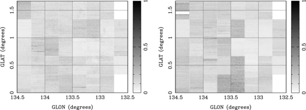
Figure 2. Gray-scale maps showing rms noise level at each pixel of the CO J = 2–1 (left) and 13CO J = 2–1 (right) emission maps. Units of intensity wedges are main beam brightness temperature in Kelvins.
Download figure:
Standard image High-resolution imageThe observing parameters are summarized in Table 1.
Table 1. Observing Parameters
| (a) CO and 13CO J = 2–1 observations | |
| Telescope angular resolution | 32'' (FWHM) |
| Final map resolution | 38'' (FWHM) |
| Field observed | l = 1325 to 1345 |
| b = 0° to +167 |
|
| Spectrometer resolution | 1.0 MHz |
| Line rest frequencies and velocity resolutions | |
| CO | 230.538 GHz; 1.30 km s−1 |
| 13CO | 220.399 GHz; 1.36 km s−1 |
| Telescope main beam efficiency | 0.73 ± 0.03 |
| Map rms noise (brightness temperature) | |
| CO | 0.12 K |
| 13CO | 0.14 K |
| (b) CO J = 3–2 observations | |
| Telescope resolution | 24'' (FWHM) |
| Map resolution | 25'' (FWHM) |
| Field observed | l = 1335 to 1340 |
| b = +10 to +133 |
|
| Spectrometer resolution | 1.0 MHz |
| Line rest frequency and velocity resolution | 345.796 GHz; 0.867 km s−1 |
| Map rms noise (brightness temperature) | 2.2 K |
Download table as: ASCIITypeset image
3. RESULTS FOR J = 2–1 LINES
3.1. Image Data
Figure 3 shows an image of the maximum main beam brightness temperature for the CO J = 2–1 line in the LSR velocity range −60 to −25 km s−1, which covers the full range of emission from the Perseus arm clouds (e.g., Heyer & Terebey 1998). (There is weak, diffuse emission at velocities near 0 km s−1 produced by local clouds, but we do not consider that in this paper.) In Figure 3, three areas of very bright CO emission stand out, and these are in the direction of three known regions of massive star formation: W3 Main, W3(OH), and AFGL 333. W3 North is another H ii region, containing a single O6 star (Feigelson & Townsley 2008) apparently associated with the W3 molecular cloud complex. In the south,2 KR 140 is a diffuse H ii region (Kallas & Reich 1980) which is probably more distant than W3 but shows evidence of star formation now occurring in a swept-up shell of gas surrounding the H ii region (Kerton et al. 2001). The magenta contours in Figure 3 show the 1420 MHz continuum emission from the CGPS (Taylor et al. 2003), which traces here mainly the emission measure of ionized gas. The brightest continuum is from the W3 Main H ii region complex, with weaker diffuse emission extending out to a distance of a degree around the peak.
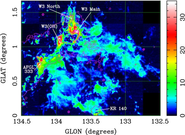
Figure 3. False color image of the CO J = 2–1 maximum line intensity for the velocity range −60 to −25 km s−1. Color wedge is labeled in Tmb (K). Highest value in this image is 53.6 K. Magenta contours show the 1420 MHz continuum emission from the Canadian Galactic Plane Survey (Taylor et al. 2003). Contour levels are at 10, 20, 50, 100, 500, and 2000 K brightness temperature, and resolution of continuum image is ∼1'. Principal H ii regions/IR sources are indicated.
Download figure:
Standard image High-resolution imageOnly ∼50% of the pixels in Figure 3 show CO emission greater than 0.5 K, which is about the 4σ level for the map and is a conservative lower limit to a detection threshold. The majority of the detected gas as seen projected on the plane of the sky has a relatively low CO J = 2–1 brightness temperature. Some 90% of the mapped area has CO peak brightness temperatures <6 K, as shown in the cumulative distribution of pixel values in Figure 4 (top left). The differential brightness temperature distribution (Figure 4, bottom left) shows a peak near 0.2 K due to the relatively large fraction (∼50%) of undetected pixels, with a nearly flat distribution extending from 1 K up to about 5.5 K, then declining toward higher temperatures. Less than 5% of the mapped area shows CO J = 2–1 emission brighter than 10 K.
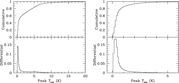
Figure 4. Normalized cumulative and differential distributions of peak Tmb for (left) CO J = 2–1 image shown in Figure 3; and (right) 13CO J = 2–1 image shown in Figure 5. The rms noise for the x-axis is 0.12 K for CO and 0.14 K for 13CO.
Download figure:
Standard image High-resolution imageFigure 5 shows an image of the maximum brightness temperature in the 13CO J = 2–1 line, over the same velocity range as for CO in Figure 3. About 70% of the area shown in Figure 5 has Tmb < 0.5 K (see Figure 4, top right), which is ∼3.5 × the rms noise level per pixel and per velocity channel in the 13CO line. Only 10% of the pixels in the 13CO map have a peak brightness temperature >1.5 K.
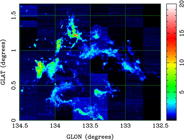
Figure 5. False color image of the 13CO J = 2–1 maximum line intensity for the velocity range −60 to −25 km s−1. Color wedge is labeled in Tmb (K). Highest value in this image is 22.8 K.
Download figure:
Standard image High-resolution imageThe integrated line intensities for CO J = 2–1 and 13CO J = 2–1 are shown in Figures 6 and 7. The emission spectrum in each pixel was summed over the velocity range −60 to −25 km s−1, which is the range of velocities associated with the Perseus spiral arm material. The images are displayed in units of Tmb × velocity (K km s−1). The integrated intensity images resemble the peak brightness temperature images (Figures 3 and 5). The integrated emission in both CO isotopologues is dominated by the three bright CO emission regions associated with W3 Main, W3(OH), and AFGL 333.
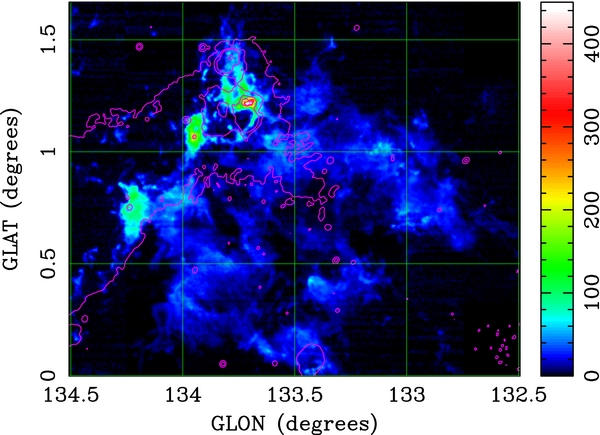
Figure 6. False color image of the CO J = 2–1 integrated line intensity, over the velocity range −60 to −25 km s−1. Color wedge is labeled in (Tmb × velocity) (K km s−1). Maximum integrated intensity in this image is 495 (K km s−1). Magenta contours show the 1420 MHz continuum emission from the Canadian Galactic Plane Survey (Taylor et al. 2003). Contour levels are at 5, 10, 25, 50, 500, 2500 K brightness temperature, and resolution of continuum image is ∼1'.
Download figure:
Standard image High-resolution image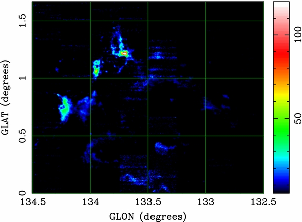
Figure 7. False color image of the 13CO J = 2–1 integrated line intensity, over the velocity range −60 to −25 km s−1. Color wedge is labeled in (Tmb × velocity) (K km s−1). Maximum integrated intensity in this image is 148 (K km s−1).
Download figure:
Standard image High-resolution imageHistograms of the distributions of integrated intensities for both CO and 13CO are shown in Figure 8. The majority of pixels have low integrated line intensities relative to the peak in each image. For CO J = 2–1, about 80% of the image has integrated intensities <50 K km s−1, and for 13CO J = 2–1, a similar fraction has integrated intensity <10 K km s−1.
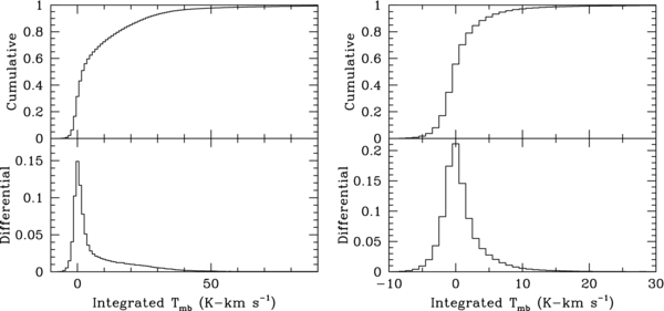
Figure 8. Normalized cumulative and differential distributions of integrated Tmb for (left) CO J = 2–1 image shown in Figure 6 and (right) 13CO J = 2–1 image shown in Figure 7.
Download figure:
Standard image High-resolution image3.2. Velocity Channel Maps
The gas kinematics are illustrated in Figures 9 and 10, which show the CO and 13CO J = 2–1 brightness temperature distributions averaged in 2 km s−1 wide velocity intervals over the range from −54.5 to −31 km s−1. This range covers essentially all the significant emission. Figure 9 shows that the CO emission is produced in very complex spatial structures which change dramatically with velocity across the line. There are areas of extended diffuse emission as well as many compact, barely resolved clumps. At 2.0 kpc, the distance to W3, the resolution of these maps (38'') corresponds to a linear size of 0.4 pc, so the numerous barely resolved features in the velocity channel maps must be subparsec in size.
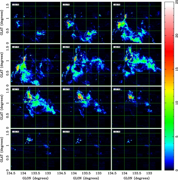
Figure 9. False color image of the CO J = 2–1 maps averaged over 2 km s−1 velocity intervals. Color wedge is labeled in K-Tmb. Number in upper left of each panel gives the mean LSR velocity. Download the high-resolution figures from the electronic edition and zoom in to see the full range of detail in the images.
Download figure:
Standard image High-resolution image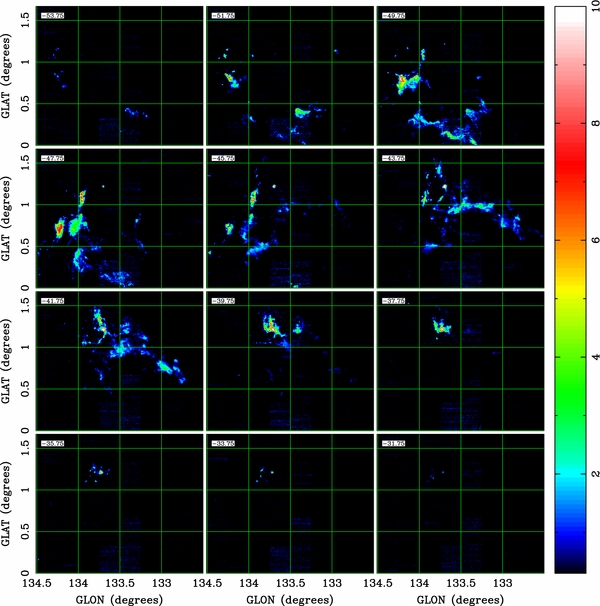
Figure 10. False color image of the 13CO J = 2–1 maps averaged over 2 km s−1 velocity intervals. Color wedge is labeled in K-Tmb. Number in upper left of each panel gives the mean LSR velocity. Download the high-resolution figures from the electronic edition and zoom in to see the full range of detail in the images.
Download figure:
Standard image High-resolution imageThere is an overall gradient of the spatial distribution with velocity. The most negative emission, with VLSR < −46 km s−1, is mainly confined to roughly the southern half of the field. Diffuse emission to the southwest of W3 Main appears at higher velocities with VLSR > −46 km s−1. The brightest CO emission peaks lie along a line from SE to NW from AFGL 333 through W3(OH) to W3 Main/W3 North, a locus of clouds that was named the high density layer (HDL) by Lada et al. (1978; see also Megeath et al. 2008). The most negative velocities are in the vicinity of AFGL 333 and W3(OH). W3 Main and W3 North have the most redshifted CO of the HDL peaks, as Lada et al. (1978) noted from their low-resolution study. The W3 Main region has significantly broader lines than other positions in the map, consistent with the high level of massive star formation that has recently occurred there.
The corresponding velocity channel maps for 13CO J = 2–1, in Figure 10, show the same trends as seen in Figure 9, but there are many more blank pixels because the 13CO line is generally weaker and detected in fewer sight lines. The presence of many small, barely resolved features around W3 Main at the highest velocities is notable. These may represent relatively warm, high column density clumps associated with the current active star formation in the gas surrounding the IC 1795 OB association (Oey et al. 2005), which lies between W3 Main and W3(OH).
3.3. Velocity Moment Maps
We calculated first-moment (or centroid) maps,
summed over the velocity range (− 60, −25) km s−1, where I is the intensity (brightness temperature) at pixel (x, y) and velocity channel V. Figure 11 displays the velocity centroid map for CO J = 2–1, using a different color palette from the one used for the line intensity maps. Pixels with peak Tmb < 1.3 K are blanked.
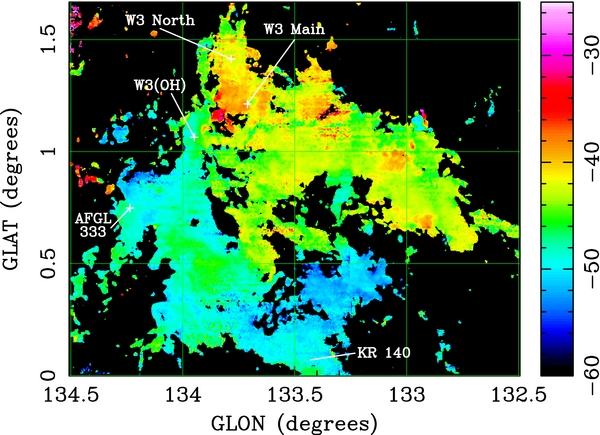
Figure 11. First moment or velocity centroid calculated between −60 and −25 km s−1 (LSR) for CO J = 2–1 emission. Color wedge is labeled in VLSR (km s−1). Pixels with peak CO Tmb < 1.3 K are blanked. Principal H ii regions/IR sources are indicated.
Download figure:
Standard image High-resolution imageThe velocity centroid map shows the overall trends in velocity gradient noted in Figures 9 and 10. The gas in the lower left is more blueshifted relative to the upper half of the map. There are notable "islands" of redshifted gas at the positions between W3 Main and W3(OH), and at (l, b) = (1344, +08), (1331, +09), and (1329, +07). The velocity gradient along the HDL from AFGL 333 to W3 North is clearly visible in the centroid map.
The velocity centroid map for 13CO is shown in Figure 12. Pixels with peak Tmb < 1.3 K are blanked. The same trends as in Figure 11 are evident but there are fewer pixels bright enough to show the full area of the clouds.
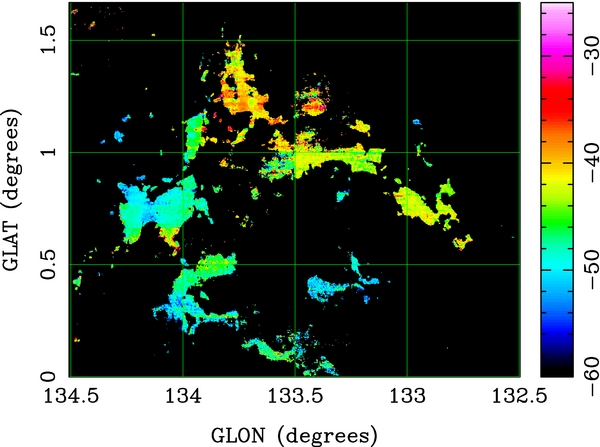
Figure 12. First moment or velocity centroid calculated between −60 and −25 km s−1 (LSR) for 13CO J = 2–1 emission. Color wedge is labeled in VLSR (km s−1). Pixels with peak 13CO Tmb < 1.3 K are blanked.
Download figure:
Standard image High-resolution imageWe also calculated the second moment (or velocity dispersion) of the spectra at each map pixel,
The typical second-moment dispersions are 3–4 km s−1, corresponding to a typical Gaussian FWHM line width of ∼7 km s−1 for both CO and 13CO. A small fraction of pixels show second-moment values up to ∼12 km s−1, mainly in the direction of W3 Main. There the line profiles are typically not well represented by a single Gaussian component, indicating that the gas is kinematically disturbed by the associated massive stars and H ii regions.
3.4. CO/13CO Ratio Maps
We have constructed maps of the CO/13CO J = 2–1 calibrated line intensity ratios from the data sets presented above. Our data are especially well suited for this kind of analysis because both isotopologues are observed simultaneously through the same telescope optics, so the registration of the two images is guaranteed, even if there are telescope pointing errors (which we argue are small in any case). The intrinsic angular resolutions of the observations differ by the ratio of the line frequencies, and we correct for this difference by convolving the raw maps with appropriate kernel functions to put both isotopologues at an effective resolution of 38'' (FWHM), as described in Section 2. The intensity ratio may be a useful diagnostic of the mean CO optical depth within a map resolution element. If, for example, the intrinsic ratio of abundances is f12/13 = n(CO)/n(13CO), where n(X) is the density of molecular species X, and if we can assume that the abundance ratio is constant within a molecular cloud, then the ratio of line optical depths through the cloud will have this same ratio, provided CO and 13CO have the same excitation conditions at each point in the cloud. If so, then the ratio, R, of observed line brightness temperatures (neglecting any background continuum) should be
An estimate of the 12C/13C isotope ratio in the interstellar gas is 50 ± 10 (Milam et al. 2005). Taking f12/13 = 50, the observed line intensity ratio can be used to estimate τCO and  . For example, a ratio of R = 10 would imply τCO(J = 2–1) ≈ 5 for the simple homogeneous cloud model. R = 3 gives τCO(J = 2–1) = 20, and R = 1.58 would imply τCO(J = 2–1) = 50 and therefore
  , i.e., the 13CO J = 2–1 line is becoming optically thick for R ⩽ 1.6.
In more realistic models, a low line ratio (even R ⩽ 1) may result from self-absorption by cold foreground gas with high CO opacity but low excitation temperature. A fully quantitative interpretation of the J = 2–1 line ratio requires a statistical equilibrium/radiative transfer calculation for a specific molecular cloud model. Line ratio images can nevertheless be useful for identifying positions and velocities with high line optical depths and/or CO self-absorption, and for estimating initial conditions in constructing such detailed cloud models.
Figure 13 shows images of the J = 2–1 line intensity ratio, R, averaged in 2 km s−1 wide velocity bins, for the same set of velocities as are shown in Figures 9 and 10. Pixels where the 13CO brightness temperature is <0.75 K, which is ∼5 times the rms noise level, are blanked out. Figure 13 uses a different color palette than Figures 9 and 10. Magenta indicates regions of low R implying large CO line optical depth. Areas shown in gray have R < 1.6, where the 13CO line may also be optically thick. Areas shown in white have R < 1, indicating likely cases of self-absorption in the CO J = 2–1 line.
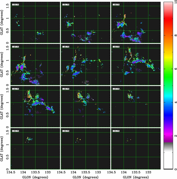
Figure 13. False color images of the J = 2–1 CO/13CO line intensity ratio averaged over 2 km s−1 velocity intervals. Color wedge is labeled in Tmb(CO)/Tmb(13CO) ratio values. Ratios less than 1.6 are in gray and may have optically thick 13CO emission. Areas in white shading from gray have the line ratio less than unity, probably indicating that the CO line is self-absorbed. Pixels are blanked where Tmb(13CO) is less than 0.75 K (∼5σ). Number in upper left of each panel gives the mean LSR velocity, as in Figures 9 and 10. Download the high-resolution figures from the electronic edition and zoom in to see the full range of detail in the images.
Download figure:
Standard image High-resolution image3.5. Comparison with BOLOCAM 1.1 mm Continuum Image
The relationship between molecular line emission and thermal dust continuum emission is of great importance in understanding the properties of interstellar matter and the processes which lead to star formation from that matter. Ruch et al. (2007) and Polychroni et al. (2010) have presented Spitzer images from the four IRAC bands as well as MIPS 24 μm results. Ruch et al. (2007) focus on the point sources detected by Spitzer and find that the area lying between W3 Main and W3(OH) contains a large concentration of very young stars, mainly of class I and II, which they call the Central Cluster. The cluster lies in a cavity, with low dust/gas content, and is surrounded by a denser shell that includes the currently active star-forming regions W3 Main and W3(OH). Ruch et al. (2007) argue that this disposition of young stars, gas, and dust is consistent with a scenario of triggered star formation which initiated the formation of the Central Cluster and the ongoing massive star formation now creating the H ii regions in the shell. Polychroni et al. (2010) present Spitzer and JCMT CO J = 3–2 data for a larger region complementing Ruch et al. (2007). They derive star formation efficiencies which indicate that the parts of the molecular cloud which appear to be undergoing triggered star formation have much higher star formation efficiencies than the more quiescent parts.
Besides the Spitzer observations, another important new data set showing millimeter-wavelength continuum emission in the W3 region is the recently released BGPS (Aguirre et al. 2011; Rosolowsky et al. 2010). The 1.1 mm continuum is dominated by thermal emission from cold dust, except in the direction of high emission measure H ii regions where free–free bremsstrahlung may also be a significant contribution. In this section, we draw some comparisons between the BGPS results and our molecular line maps.
Figure 14 displays the peak line intensity, Tmb, for the 13CO J = 2–1 line, regardless of velocity, as in Figure 5 but with a different color palette to contrast better with the cyan contours which show the 1.1 mm continuum emission from the BGPS. The BGPS data were smoothed slightly from their original 33'' (FWHM) resolution to match the 38'' resolution of the CO maps. The resulting rms noise level of the 1.1 mm continuum map is 0.025 Jy beam−1. It is evident in Figure 14 that only a modest fraction of the molecular gas detected in this field is also detected in the BGPS as 1.1 mm dust continuum emission. The 13CO line intensity is determined by the gas column density as well as the 13CO excitation temperature. The relatively good correspondence between the 13CO peak intensity and the BGPS contours in Figure 14 illustrates how the 1.1 mm continuum generally picks out the highest column density lines of sight.
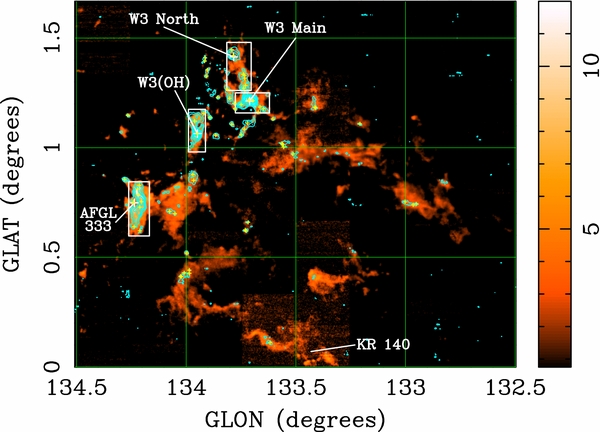
Figure 14. Color: 13CO J = 2–1 peak line intensity, as in Figure 5 but with a different color palette to contrast better with the overlaid contours; color wedge is labeled in Tmb (K). Contours: 1.1 mm continuum emission intensity from the BOLOCAM Galactic Plane Survey. Contours are at 0.1, 0.25, 0.5, 1, 2.5, 5, and 10 Jy beam−1. The BOLOCAM image has been smoothed slightly by convolution to match the CO map resolution of 38'' (FWHM). The rms noise level in the continuum map is about 0.025 Jy beam−1 for this field. Small yellow crosses mark the peak positions of the 65 cataloged BGPS sources in this field, from Rosolowsky et al. (2010), for which Gaussian fits to the 13CO J = 2–1 spectra were made (see Table 2). Labeled white crosses with rectangles show the regions selected for correlation plots in Figure 16.
Download figure:
Standard image High-resolution imageTo quantify this correspondence, we have extracted all the sources from the BGPS catalog (Rosolowsky et al. 2010) that lie within the CO map area. There are 66 objects listed though we found one pair (Nos. 7340/7341) which were weak and probably redundant sources (separated by 19'' or one-half the map resolution), leaving 65 independent BGPS sources in our mapping field. The peak positions of these objects are marked with small yellow crosses in Figure 14. Table 2 lists the BGPS sources, including the galactic coordinates of the peak position and S40, the 1.1 mm continuum flux density within a 40'' diameter aperture, which nearly matches the 38'' FWHM resolution of our CO and 13CO maps. The S40 values in Table 2 have not been multiplied by the factor of 1.5 suggested in the BGPS catalog description, but are simply the values as given in the catalog. The integrated 13CO intensity at each BGPS source position was extracted from the image in Figure 7 and is listed in Column 5 of Table 2.
Table 2. 13CO (J = 2–1) Line Properties at BGPSa Source Positions
| 13CO Gaussian Fit Parameters | |||||||||
|---|---|---|---|---|---|---|---|---|---|
| BGPS | lmax | bmax | S40b | 13CO Inten. | Fit | Ampl. | Vpeakc | FWHM | Fit rms |
| No. | (°) | (°) | (Jy) | (K km s−1) | Comp. | (K) | (km s−1) | (km s−1) | (K) |
| 7336 | 132.951 | 0.743 | 0.111 | 12.1 | 1 | 4.31 | −41.9 | 2.6 | 0.07 |
| 7337 | 132.965 | 0.739 | 0.101 | 11.7 | 1 | 4.05 | −42.1 | 2.7 | 0.10 |
| 7338 | 133.001 | 0.753 | 0.192 | 13.0 | 1 | 3.95 | −43.3 | 2.9 | 0.07 |
| 7339 | 133.207 | 1.109 | 0.100 | 6.6 | 1 | 2.28 | −41.8 | 2.4 | 0.08 |
| 7340 | 133.409 | 1.181 | 0.111 | 23.8 | 1 | 5.11 | −40.5 | 3.2 | 0.42 |
| 7342 | 133.513 | 0.971 | 0.120 | 13.1 | 1 | 2.96 | −42.6 | 3.7 | 0.29 |
| 7343 | 133.555 | 1.003 | 0.097 | 9.0 | 1 | 1.51 | −44.7 | 3.4 | 0.13 |
| 9.0 | 2 | 1.89 | −41.1 | 2.4 | |||||
| 7344 | 133.559 | 1.015 | 0.097 | 14.9 | 1 | 1.36 | −44.3 | 3.4 | 0.21 |
| 14.9 | 2 | 2.03 | −40.8 | 3.0 | |||||
| 7345 | 133.563 | 1.019 | 0.126 | 10.0 | 1 | 0.72 | −45.4 | 3.2 | 0.12 |
| 10.0 | 2 | 2.21 | −40.7 | 3.0 | |||||
| ⋅⋅⋅ | |||||||||
Notes. aRosolowsky et al. (2010). bFluxes have not been scaled by any correction factor (cf. Rosolowsky et al. 2010). cLocal Standard of Rest.
Only a portion of this table is shown here to demonstrate its form and content. A machine-readable version of the full table is available.
Download table as: DataTypeset image
Since the BGPS sources are from a continuum survey, therefore lacking in kinematic information, we have examined the 13CO spectra at each of the 65 source positions to extract emission line velocities, intensities, and line widths associated with the continuum sources. We used a standard Gaussian component fitting algorithm (task gaufit in the MIRIAD software package). Most sources were adequately fit by a single Gaussian component, i.e., the rms of the residual to the fit was <0.2 K, comparable to the overall map rms. In these cases, Column 6 of Table 2 is set to 1, and Columns 7–9 give the amplitude and velocity of the Gaussian peak, and the FWHM. The last column of Table 2 gives the rms of the residual to the fit. In 12 cases, the 13CO line was clearly non-Gaussian, so we allowed two independent Gaussian components to obtain an adequate fit. In these cases, Column 6 lists the component number, with the amplitude and velocity of the component peak and the FWHM in Columns 7–9. Column 10 gives the rms of the residuals for the sum of the components.
The Gaussian fit parameters are only an approximate description of the line shapes. Where a single component gives a good fit to the 13CO line profile, or where two well-separated components are present, then the center velocities and widths are probably good representations of the cloud kinematics. For BGPS source positions where blended Gaussian components are needed for an adequate fit, the physical interpretation of the fit parameters is not so clear. The individual components may not correspond to physically distinct clouds viewed along the same line of sight but rather to complex cloud kinematics.
The component center velocities (Vpeak) in Table 2 are distributed broadly between −53 and −35 km s−1. The distribution of component velocities in galactic coordinates is shown in Figure 15. The large-scale gradient noted in Section 3.3 above, on velocity moments, is evident in the Gaussian component velocities. The more negative velocities are concentrated at lower latitude and higher longitude, with the gradient most noticeable in the right side of Figure 15, which displays velocity versus longitude.
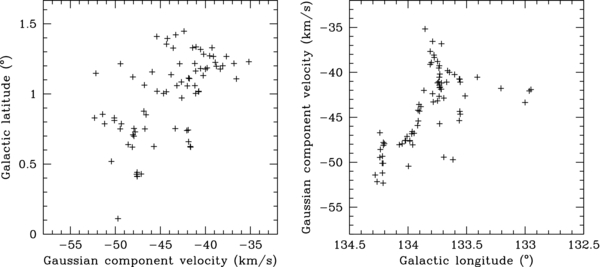
Figure 15. Left: distribution of BGPS source galactic latitudes vs. Gaussian component velocities (LSR). Right: distribution of 13CO Gaussian component velocities (LSR) vs. BGPS source galactic longitude. Data are from Table 2. Note that the figures are in position–velocity and velocity–position order, respectively.
Download figure:
Standard image High-resolution imageIf molecular gas and dust are well mixed, one would expect that sight lines with relatively strong 13CO emission should also exhibit detectable 1.1 mm dust continuum. However, comparison of BGPS map intensities with the 13CO line emission must also consider the spatial filtering effect of the BOLOCAM survey method (Rosolowsky et al. 2010; Aguirre et al. 2011). The BGPS catalog description states that 90% of the total source flux is spatially filtered out for structures with sizes > 5 9, and 50% is lost for sizes > 38. In contrast, the OTF scanning technique we used for the spectral line maps recovers all of the line flux at each pixel. We might also expect that there is a range of physical properties in the clouds associated with the BGPS sources (though spatial filtering may also have an effect). To examine the role of source properties we graphed pixel-by-pixel correlation diagrams of the BGPS intensity (in Jy beam−1) versus the 13CO integrated line intensities for spatially limited regions associated with the brightest H ii regions in the field. Pixels with BOLOCAM intensity <3σ (0.075 Jy K−1) are omitted. (Bieging et al. 2010 made similar correlation plots for selected areas in the W51 field and found relatively tight but nonlinear correlations for limited regions around BGPS peaks, and for limited velocity ranges.) In Figure 16, we show four examples of such correlation plots, for the rectangular boxes labeled in Figure 14.
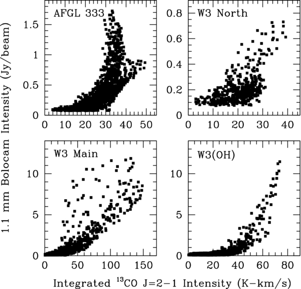
Figure 16. Pixel-by-pixel correlation plot of integrated 13CO J = 2–1 intensity (K km s−1, as in Figure 7) vs. BOLOCAM BGPS intensity (Jy beam−1) for the four regions outlined in Figure 14. Pixels with BOLOCAM fluxes <3σ (0.075 Jy beam−1) have been omitted.
Download figure:
Standard image High-resolution imageAFGL 333. This region was identified with IRAS 02245+6115 by Carpenter et al. (2000) as a compact cluster of ∼120 stars with a far-IR luminosity of 3300 L☉. (The IRAS source position is marked by a white cross in Figure 14.) Their CO and 13CO J = 1–0 maps agree well with our J = 2–1 maps, which show that the stellar cluster lies in a "bay" to the east of a molecular ridge that coincides with a ridge of 1.1 mm continuum. There is a ∼10σ BGPS continuum source (marked by small yellow cross) very close to the cluster center, which is at a local minimum in the 13CO intensity (Figure 14). The plot in Figure 16 shows some correlation between the 13CO and 1.1 mm continuum, but for the x-axis range from ∼30 to 40 K km s−1, the continuum is essentially uncorrelated with the line emission. Although the line and continuum emission fall along the same ridge to the west of the AFGL 333 cluster, the intensities do not track in detail. This behavior may be related to heating effects on the dust from the cluster stars. The sharp boundary apparent on the lower right in the distribution of points in Figure 16 may be an artifact resulting from the spatial filtering of the BOLOCAM images.
W3 North. The 13CO and 1.1 mm continuum are much weaker in this region than in W3 Main or W3(OH), and exhibit only a modest correlation. Figure 14 shows that the H ii region associated with the isolated O6 V exciting star (Oey et al. 2005; Feigelson & Townsley 2008; marked by a white cross) is not a well-defined 13CO peak. There is, however, a "spur" of emission extending north from W3 Main that appears to connect with the W3 North H ii region. This part of the rectangular region outlined in Figure 14 is responsible for the greatest part of the correlation seen in Figure 16. The local maxima in the 13CO and 1.1 mm continuum, lying between W3 Main and W3 North, may be potential sites of future star formation.
W3 Main. This region contains the brightest radio and mm continuum, associated with the massive forming OB cluster that ionizes the gas, heats the dust, and disrupts the parent molecular cloud. The relatively poor correlation in Figure 16, compared to W3(OH), is therefore not surprising. There is a well-defined lower envelope to the distribution of points, and a locus concentrated just above the lower boundary that is similar to the trend seen for W3(OH), but between 30 and 130 K km s−1 on the x-axis, there are many pixels with 1.1 mm intensities showing little correlation with the 13CO intensity. The large scatter probably results from a contribution by free–free emission to the 1.1 mm continuum toward the bright H ii regions.
W3(OH). The best correlation is for the region around W3(OH), an ultracompact (UC) H ii region at the southern end of the molecular shell that extends from W3 Main around the IC 1795 OB association. Comparison of the 1.1 mm continuum contours with the 13CO J = 2–1 integrated intensity in Figure 14 shows that the continuum follows the 13CO closely, with both having maxima at the position of W3(OH) (white cross in Figure 14). This good correlation suggests that the UC H ii region has not significantly disrupted its parent molecular cloud, and does not contribute significant free–free emission to the 1.1 mm continuum. The distribution of points in Figure 16 intersects the x-axis at ∼30 K km s−1, similar to the examples presented by Bieging et al. (2010) for W51, probably because the BOLOCAM image has filtered out extended low-brightness 1.1 mm continuum emission.
A number of physical effects must influence the correlations seen in Figure 16, making the interpretation of these plots less than straightforward.
- 1.The regions with higher CO J = 2–1 peak temperatures (W3 Main and W3(OH)) show larger extents in both BOLOCAM intensity and 13CO integrated intensity, compared to the regions with lower CO peak temperatures (AFGL 333 and W3 North). The CO line peak temperature is likely to be an indicator of the cloud kinetic temperature, so it is reasonable that the colder clouds show smaller spans of 13CO intensities, while the warmer regions show a larger range of 13CO values. Self-absorption in the CO line may also affect the observed peak temperature leading to an underestimate of the kinetic temperature.
- 2.The slope and linearity of the correlations in Figure 16 vary from region to region. The slope should depend, to first order, on the dust and gas temperatures. If the 13CO line is optically thin and the gas and dust are thermally well coupled, a linear relation should result as a function of line-of-sight column density for an isothermal cloud. The trends in Figure 16 should curve upward as the 13CO becomes increasingly saturated at higher column density, provided the cloud is isothermal. Another possible source of nonlinear correlations could be gradients in cloud temperature and density. At the BOLOCAM wavelength of 1.1 mm, hc/λk = 13.0 K which is comparable to the grain temperatures of interest, so the dust emission will vary more steeply than linearly with grain temperature, while the 13CO excitation temperature should vary no more than linearly with gas kinetic temperature. Therefore, we would expect a warmer cloud to produce greater 1.1 mm continuum relative to 13CO line emission for a given column density, compared to a colder cloud. The 1.1 mm continuum emission will be more strongly weighted toward dense, warm inner cores of molecular clouds compared to the 13CO line, so a set of sight lines through a range of column densities, as shown in the panels of Figure 16, would also show the upward curving trends seen in some of the example regions even if the 13CO line is optically thin throughout the cloud. Our CO/13CO line ratio maps (Figure 13) indicate that the 13CO line is just becoming optically thick at some of the BGPS source peaks. An inward temperature gradient is probably also present in the clouds, which clearly have internal heat sources. In either case, the correlations in Figure 16 should exhibit nonlinear behavior, as is in fact observed.
- 3.The scatter of points above the general trend for W3 Main is probably a result of free–free emission contributions to the 1.1 mm continuum, in addition to the thermal dust emission. The lack of correlation for AFGL 333 may be related to molecular dissociation or dynamical effects of the ionized gas, suggested by the morphology of the CO maps compared with the BOLOCAM map.
The trends in the correlations of the line and continuum data suggest that they could usefully constrain detailed cloud models in terms of gas and dust temperature distributions as well as density gradients and H ii regions, in determining molecular excitation and line profiles. Such detailed models are beyond the scope of this paper but will be undertaken in future work.
3.6. Results for J = 3–2 Line
3.6.1. Image Data
The CO J = 3–2 map of the 30' × 20'(l × b) region encompassing W3 Main and W3(OH) is shown in Figure 17, which presents the peak CO J = 3–2 line intensity within the velocity range −60 to −25 km s−1. The positions of the H ii regions are marked by the white crosses. The circle of radius 5' shows the location of the OB association IC 1795, from the photometric study of Oey et al. (2005). The yellow cross marks the dominant O star in the cluster, BD+61°411, which lies nearly centered between W3(OH) and W3 Main. Radio continuum emission at 1420 MHz from the CGPS is shown in contours as in Figure 3.
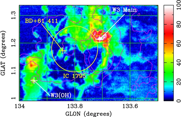
Figure 17. False color image of the CO J = 3–2 maximum line intensity for the velocity range −60 to −25 km s−1. Color wedge is labeled in Tmb (K). Highest value in this image is 117 K and rms is 2 K. Yellow circle marks the central core of OB association IC 1795, as shown in Oey et al. (2005, their Figure 3). The position of the dominant O star, BD+61°411, is marked. H ii regions are marked as in Figure 3 above. Magenta contours show the 1420 MHz continuum emission from the Canadian Galactic Plane Survey (Taylor et al. 2003). Contour levels are at 10, 20, 50, 100, 500, and 2000 K brightness temperature, and resolution of continuum image is ∼1'.
Download figure:
Standard image High-resolution imageFigure 17 shows that CO J = 3–2 emission is present at almost every pixel, above the 3σ level (6 K). The brightest CO is at the W3 Main H ii region complex, as in the CO J = 2–1 maps. In contrast, the position of the UC H ii region W3(OH) does not stand out in the CO cloud surrounding it. There is an arc of CO around the southwest half of the IC 1795 cluster and extending from W3 Main to W3(OH). A similar but clumpier arc of CO emission extends around the northeast side of IC 1795 from W3(OH) to W3 Main. These structures have the appearance of a shell of molecular gas surrounding the OB cluster.
The integrated CO J = 3–2 line intensity is shown in Figure 18. The general appearance of the emission is similar to that in Figure 17 but with greater contrast. The CO associated with W3 Main dominates the map, while the cloud around W3(OH) is a relatively minor peak. There is also at least a partial arc of CO evident on the southwest perimeter of IC 1795, but is less obvious on the northeast side.
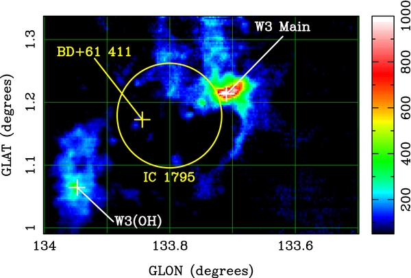
Figure 18. False color image of the CO J = 3–2 integrated line intensity, over the velocity range −60 to −25 km s−1. Color wedge is labeled in (Tmb × velocity) (K km s−1). Maximum integrated intensity in this image is 1085 (K km s−1). Symbols as in Figure 17.
Download figure:
Standard image High-resolution imageThe CO J = 3–2 images closely resemble the corresponding CO J = 2–1 maps for the same region encompassing W3 Main and W3(OH). If the CO excitation were uniform at all locations, the 3–2 and 2–1 images should be identical in appearance except for optical depth effects. Where the CO is optically thick, presumably at the peak of the emission lines, we would expect the peak brightness temperatures to be identical within a scale factor of order unity, due to the different velocity resolutions giving slightly different channel dilutions at the line peaks. In fact, we find significant variations in the ratio of peak line intensities,
across the map. Figure 19 (top) shows Tpeak(CO 3–2) after convolving Figure 17 spatially to match the 38'' (FWHM) resolution of the CO 2–1 map (Figure 3). Figure 19 (bottom) shows the above ratio for the convolved image in Figure 19 (top) divided by the CO 2–1 peak intensity from Figure 3. Pixels where the CO 2–1 peak intensity is <1 K (∼8σ) are blanked. The black contours are the same as the contours in Figure 19 (top) to show how the line ratio varies with respect to the 3–2 peak intensity. Over most of the mapped area, the peak intensity ratio is relatively uniform at around 1.4 ± 0.3. At positions on the edges of the bright CO 3–2 emission, however, the 3–2 line appears to be significantly enhanced relative to the 2–1 line, as indicated by the orange, red, and white colors. Even at these positions the emission is at least several times the rms noise level in both 2–1 and 3–2 maps. The telescope pointing is certainly better than one-half of the 10'' pixel, so we are confident that the areas with high [Tpeak(CO 3–2)]/[Tpeak(CO 2–1)] are real, not artifacts, e.g., of inaccurate registration of the two maps. Note also the relatively higher 3–2 intensity in the vicinity of the W3 Main complex of H ii regions, where both lines are strong. The areas showing up in red or white in Figure 19 (bottom) are probably locations where the molecular gas is being influenced by UV radiation from nearby OB stars or also by the more general interstellar radiation field with contributions from the various OB clusters in the W3 and W4 H ii region complex, i.e., "photon-dominated regions" or PDRs. We note that the quantitative values for intensity ratios indicated in Figure 19 (bottom) should be taken with some caution, as there may be unrecognized systematics in the overall calibration of the brightness temperature scale of the CO 3–2 data in particular. Despite possible scaling uncertainties, the patterns in Figure 19 (bottom) are suggestive of PDRs located in the interface between the dense, cold molecular gas and the hot, diffuse, UV-illuminated H ii regions which surround the molecular clouds. A detailed excitation/radiative transfer analysis of the CO lines including both the CO and 13CO 2–1 and the CO 3–2 lines could better constrain the temperature and excitation conditions in the bulk of molecular clouds as well as in these PDRs. Such an analysis will be the subject of a future study.
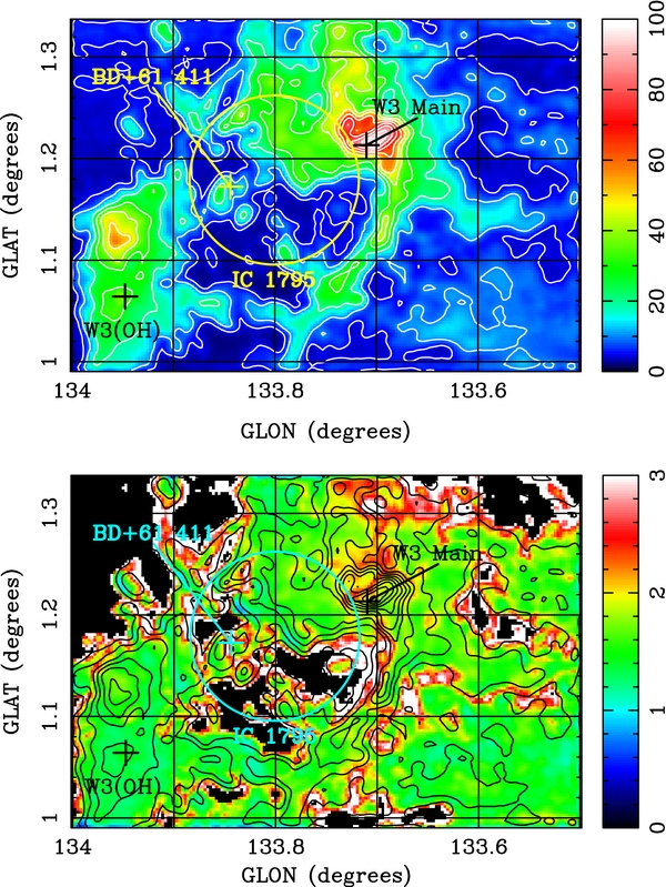
Figure 19. Top: Peak brightness temperatures for CO J = 3–2 (see Figure 17) but convolved to 38'' FWHM resolution. Color wedge is in K. Contours are overlaid at 5, 10, 20, 30, 40, 50, 60, 70, 80, 90, and 100 K, for comparison with the bottom panel. Symbols as in Figure 17. Bottom: Ratio of peak brightness temperatures for CO J = 3–2 convolved to 38'' FWHM resolution (see the top panel), divided by peak brightness temperature for CO J = 2–1 (Figure 3), for region mapped in CO J = 3–2. Pixels with Tpeak(J = 2–1) < 1 K are blanked. Contours show the J = 3–2 peak brightness temperature, as in the top panel. Symbols as in Figure 17.
Download figure:
Standard image High-resolution image3.6.2. Velocity Channel Maps
There is significant velocity structure in the CO J = 3–2 emission, as seen in the channel maps of Figure 20, which show TB averaged in 2 km s−1 wide increments from −54 to −30 km s−1 for the same 12 velocities as the CO and 13CO J = 2–1 channel maps in Figures 9 and 10. The 3–2 channel maps are very similar to the 2–1 maps, but show some structures more clearly because of the higher angular resolution. The same large-scale gradient from W3(OH) to W3 Main is apparent. The arc of emission around IC 1795 shows up in segments over a range of velocities, encircling the OB cluster and, on opposite ends of the elliptical arcs exhibiting strong CO emission at W3 Main and W3(OH) in distinctly separate velocity channels. The small clumps of CO projected on the center of IC 1795 (yellow circle in Figure 20) show up at the most redshifted velocities, consistent with being portions of a shell on the far side of the OB association and expanding outward and away from us. There are elongated structures in some of the clumps that appear to extend radially away from the O6.5 star BD+61°411 (yellow cross) at velocities from −35.75, −33.75, and −31.75. This morphology is suggestive of some kind of interaction between the O star and the dense molecular gas in the clumps, possibly via radiation or a stellar wind, though it is not possible to determine the location of these clumps along the line of sight relative to the O star. Their proximity as seen in the plane of the sky may suggest a spatial association but that cannot be proven from these data alone.
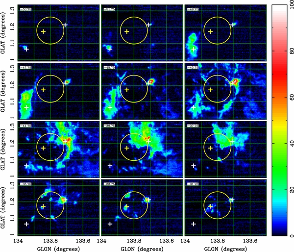
Figure 20. False color image of the CO J = 3–2 maps averaged over 2 km s−1 velocity intervals. Color wedge is labeled in K-Tmb. rms is 1.7 K pixel−1. Number in upper left of each panel gives the mean LSR velocity. Symbols as in Figure 17.
Download figure:
Standard image High-resolution image3.6.3. Velocity Moment Maps
The first moment or velocity centroid for the CO J = 3–2 map is in Figure 21. The low-level horizontal striping is an artifact of residuals to the fitted spectroscopic baselines, probably due to weather-caused fluctuations in the sky brightness during the OTF scanning. Such residual errors in the spectroscopic baselines are accentuated in the velocity moments. Nevertheless, the overall structure and velocity values agree well with the corresponding region in the CO J = 2–1 first-moment map (Figure 11). The trend from W3(OH) to W3 Main is identical and the sharp local gradient across the position of W3 Main is seen in both transitions, suggestive of a large-scale bipolar outflow or asymmetric expansion centered on the main H ii region complex. We also see the clumpy gas projected near BD+61°411 in the most redshifted centroid velocities, consistent with the channel maps of Figure 20. Our centroid map appears to be consistent with the data of Polychroni et al. (2010) who present a three-color-coded intensity map of CO J = 3–2 emission made with the JCMT. Their map is not a true velocity centroid map but shows the same trends in velocity over the region displayed in Figure 21.

Figure 21. First moment or velocity centroid calculated between −60 and −25 km s−1 (LSR) for CO J = 3–2 emission. Color wedge is labeled in VLSR (km s−1). Pixels with peak CO Tmb < 7 K ∼4σ) are blanked. Symbols as in Figure 17.
Download figure:
Standard image High-resolution image
We also calculated the second-moment map for the CO 3–2 spectra, which is a measure of the line width at each position in the field. The distribution of second moments is comparable to that found for the CO 2–1 line (see Section 3.3). The mean value is 4.2 km s−1 with a long tail to higher values, where the larger line widths are associated with the molecular gas near the W3 Main H ii region complex. Thus, the kinematics inferred from the CO 3–2 line are similar to those for the 2–1 line, as expected.
4. FITS IMAGE FILES
The calibrated brightness temperature image cubes of the CO and 13CO J = 2–1, and the CO J = 3–2 line emission are available for download in FITS format from this URL: mira.as.arizona.edu/~jbieging/W3/ or by contacting the authors.
5. SUMMARY
We have presented the results of a program at the Arizona Radio Observatory 10 m HHT on Mt. Graham, AZ, to map the molecular clouds toward the H ii region complex W3. The maps cover a 200 × 167 section of the galactic plane and span −70 to −20 km s−1 (LSR) in velocity. The data set comprises fully sampled images of the CO and 13CO J = 2–1 lines with 38'' (FWHM) resolution, calibrated in main beam brightness temperature with a calibration accuracy of <10%. The velocity resolution is ∼1.3 km s−1. The velocity range of the images includes all the gas in the Perseus spiral arm.
The typical rms noise per spectral channel is 0.10 K-Tmb for the 13CO image cube and 0.16 K-Tmb for CO. We present color figures displaying the peak line brightness temperature, the velocity-integrated intensity, and 2 km s−1 channel-averaged maps for both isotopologues. We also show maps of the CO/13CO J = 2–1 line intensity ratio as a function of velocity, and the first moment or velocity centroid. The CO and 13CO line intensity image cubes are made available in standard FITS format as electronically readable tables.
We also present a map of CO J = 3–2 emission over the 30' × 20' area containing the W3 Main and W3(OH) H ii regions and associated molecular clouds. The velocity coverage is the same as for the J = 2–1 maps, but with 0.8 km s−1 resolution and 24'' angular resolution. Comparison of the J = 3–2 maps with the CO J = 2–1 maps shows areas where the higher-J line is enhanced relative to the average line intensity ratio. These regions are located on the sides of the strong CO emission features and also in the region around the W3 Main complex of bright H ii regions. We suggest that these areas of enhanced CO J = 3–2 emission trace PDRs created in the interfaces between the dense, cold molecular clouds and the hot, UV-illuminated H ii regions.
We compare our molecular line maps with the 1.1 mm continuum image from the BGPS (Aguirre et al. 2011; Rosolowsky et al. 2010). From our 13CO J = 2–1 image cube, we derive kinematic information for the 65 BGPS sources in the mapped field, in the form of Gaussian component fits to the 13CO spectra at the position of each BGPS continuum source. Pixel-by-pixel comparisons of the 1.1 mm continuum surface brightness with the integrated 13CO line intensity for small regions containing the main continuum sources and molecular clouds show good correlations in some cases. Differences in the shapes of these correlations from one spatial region to another probably result from different physical conditions or structure in the clouds.
The data sets presented in this Supplement article provide a significant resource for further detailed analysis via cloud modeling and radiative transfer calculations, that can be combined with other results for CO lines as well as dust and free–free continuum maps. We show preliminary comparisons with the BGPS images indicating significant but nonlinear correlations between the 1.1 mm continuum and the 13CO J = 2–1 line. The morphology of the CO maps appears to support previous suggestions that the IC 1795 OB association has formed a swept-up ellipsoidal shell of molecular gas now expanding outward. Concentrations of gas along the major axis of the spheroid are the sites of current massive star formation at W3 Main and W3(OH). Finally, comparison of our CO J = 3–2 and 2–1 maps shows many features with enhanced emission in the J = 3–2 line which appear predominantly on the outer parts of the molecular clouds and, we argue, are tracing PDRs in the interfaces to the ionized gas. The molecular line maps made available here should provide strong constraints on future modeling of the many processes occurring in this beautiful example of star formation in a giant molecular cloud.
The Heinrich Hertz Submillimeter Telescope is operated by the Arizona Radio Observatory, a part of Steward Observatory at The University of Arizona. This work was supported in part by National Science Foundation grant AST-0708131 to The University of Arizona. The Canadian Galactic Plane Survey (CGPS) is a Canadian project with international partners. The Dominion Radio Astrophysical Observatory is operated as a national facility by the National Research Council of Canada. The CGPS is supported by a grant from the Natural Sciences and Engineering Research Council of Canada.
Footnotes
- 1
All velocities in this paper refer to the Local Standard of Rest.
- 2
Throughout this paper, we use the cardinal directions in terms of galactic coordinates, i.e., north and south refer to higher and lower latitude, and east and west to higher and lower longitude.